benthic cover
about
2.1 Reformat raw benthic cover data
2.2 Cross-reference benthic codes
2.3 percentage cover of main benthic categories
2.4 percentage cover of coral genera
2.5 percentage cover of coral species
2.6 percentage cover of coral trait groups
2.7 percentage cover of algae taxa
2.8 percentage cover of sponge morphs
2.9 percentage cover of zoanthids and gorgonians
2.10 percentage cover of other benthic categories
VI Reef Resilience Study
(Any Others?)
NoteWhat this page covers
This page catalogs the 50 USVI Reef Resilience Study (RRS) reef sites and maps their locations. It reads the site master catalog, which holds the static per-site variables (latitude, longitude, depth, distance from shore, and rugosity) for every site across the three monitoring programs (TCRMP, VINPS, CSUN). It renders an interactive map for exploring the full network, a site table, and a set of static island maps used in workshops.
Data used: the site master catalog 00_RRS_siteMaster_allSites_data.csv (50 sites, 16 columns) and its metadata file, both from RRSdata/00_RRS_dataCatalogStatus/.
Outputs: this page displays the catalog and its maps. It writes no derived data files. The site master CSV and its metadata are offered as downloads at the bottom.
Key figures and table: the interactive site map (Figure 1), the scrollable site catalog table, and the static island maps (the maps below).
This is an About page, so it carries no program time series. The interactive map is already an interactive-viz feature; the static island maps are candidates for a site-picker viewer.
The interactive map in Figure 1 shows the full site network. Each point is one reef site, colored by monitoring program. Hover or click a site to read its name, the year surveys began, depth, distance from shore, and rugosity.
Interactive dashboard
Explore the full site master catalog. The plot compares mean site depth across islands; the table is the complete catalog (every site and column), searchable and filterable.
Site catalog
The site master catalog holds one row per site with the static variables the study uses across every analysis: latitude and longitude, depth, distance from shore, and rugosity. We load it into dat and read its metadata into metadat.
The scrollable table below lists all 50 sites with their program, location, and physical attributes. Scroll horizontally to see every column.
Show code
dat <- read.csv("../../../RRSdata/00_RRS_dataCatalogStatus/00_RRS_siteMaster_allSites_data.csv")
metadat <- readLines("../../../RRSdata/00_RRS_dataCatalogStatus/00_RRS_siteMaster_allSites_metadata.txt")

kbl(dat[,1:11]) |>
  kable_paper(full_width = F) |>
  kable_styling(fixed_thead = T,
                bootstrap_options = c("hover", "condensed"),
                font_size = 8) |>
scroll_box(width = "200%", height = "600px")| program | site | site_code | island | yearadded | lat | lon | depth | dist_from_shore | rugosity | rugosity_year |
|---|---|---|---|---|---|---|---|---|---|---|
| TCRMP | Great Pond | GRP | STX | 2003 | 17.71097 | -64.65221 | 4.0000 | 1267.471121 | 1.104118 | 2011 |
| TCRMP | Brewers Bay | BWR | STT | 2002 | 18.34403 | -64.98435 | 6.0000 | 165.606733 | 1.587997 | 2011 |
| TCRMP | Fish Bay | FSB | STJ | 2002 | 18.31417 | -64.76408 | 6.0000 | 122.463857 | 1.265016 | 2011 |
| TCRMP | Castle | CST | STX | 2003 | 17.76278 | -64.59743 | 7.0000 | 637.673130 | 1.403704 | 2011 |
| TCRMP | Coculus Rock | CKR | STT | 2002 | 18.31257 | -64.86058 | 7.0000 | 529.220716 | 1.229097 | 2011 |
| TCRMP | Magens Bay | MGN | STT | 2002 | 18.37425 | -64.93438 | 7.0000 | 157.792267 | 1.732995 | 2011 |
| CSUN | West Little Lameshur | WLLB | STJ | 1992 | 18.31726 | -64.72780 | 7.0000 | 21.420965 | NA | NA |
| VINPS | VIIS-Newfound | VIIS_NF | STJ | 1999 | 18.34866 | -64.66778 | 7.9248 | 122.916575 | 1.521400 | 2016 |
| TCRMP | Botany Bay | BTY | STT | 2002 | 18.35738 | -65.03442 | 8.0000 | 211.805356 | 1.341732 | 2011 |
| TCRMP | Sprat Hole | SPH | STX | 2002 | 17.73400 | -64.89540 | 8.0000 | 584.285384 | 2.377433 | 2011 |
| VINPS | VIIS-Haulover | VIIS_HA | STJ | 2003 | 18.35126 | -64.67950 | 8.2296 | 87.703086 | 1.658000 | 2015 |
| TCRMP | Black Point | BPT | STT | 2003 | 18.34450 | -64.98595 | 9.0000 | 77.608439 | 1.385281 | 2011 |
| TCRMP | Coral Bay | CRB | STJ | 2011 | 18.33797 | -64.70402 | 9.0000 | 307.107221 | 1.426478 | 2011 |
| TCRMP | Savana | SVN | STT | 2003 | 18.34064 | -65.08205 | 9.0000 | 3645.055599 | 1.348563 | 2011 |
| CSUN | Yawzi | YZ | STJ | 1987 | 18.31507 | -64.72551 | 9.0000 | 50.192069 | NA | NA |
| CSUN | Cabritte Horn | CH | STJ | 1992 | 18.30714 | -64.72164 | 9.0000 | 33.063510 | 1.221674 | 2014 |
| CSUN | East Tektite | ETK | STJ | 1992 | 18.31096 | -64.72182 | 9.0000 | 8.835786 | NA | NA |
| CSUN | Europa Bay | EUR | STJ | 1992 | 18.31674 | -64.72999 | 9.0000 | 90.254080 | 1.158487 | 2014 |
| CSUN | Neptunes Table | NPT | STJ | 1992 | 18.31255 | -64.72301 | 9.0000 | 40.655130 | NA | NA |
| CSUN | White Point | WP | STJ | 1992 | 18.31445 | -64.73131 | 9.0000 | 47.697333 | NA | NA |
| VINPS | BUIS-Western Spur and Groove | BUIS_WSG | STX | 2000 | 17.79941 | -64.63618 | 9.4488 | 4234.306588 | 1.199000 | 2007 |
| TCRMP | Cane Bay | CBS | STX | 2002 | 17.77388 | -64.81350 | 10.0000 | 254.920163 | 1.865841 | 2011 |
| TCRMP | Eagle Ray | EGR | STX | 2002 | 17.76150 | -64.69880 | 10.0000 | 817.330706 | 1.230098 | 2011 |
| TCRMP | Salt River West | SRW | STX | 2002 | 17.78530 | -64.75940 | 11.0000 | 501.441926 | 1.286167 | 2011 |
| VINPS | VIIS-Yawzi | VIIS_YZ | STJ | 1999 | 18.31387 | -64.72586 | 11.2776 | 174.884932 | 1.587100 | 2015 |
| TCRMP | Flat Cay | FLC | STT | 2003 | 18.31822 | -64.99104 | 12.0000 | 2058.986891 | 1.445378 | 2011 |
| VINPS | SARI-Salt River | SARI | STX | 2012 | 17.78522 | -64.75943 | 12.0000 | 491.611818 | 1.720700 | 2012 |
| VINPS | BUIS-South Fore Reef | BUIS_SFR | STX | 2002 | 17.78455 | -64.60935 | 12.4968 | 2616.878649 | 1.560300 | 2015 |
| VINPS | VIIS-Mennebeck | VIIS_MB | STJ | 2000 | 18.35354 | -64.68437 | 13.7160 | 65.925772 | 1.752000 | 2015 |
| TCRMP | Buck Island STT | BIT | STT | 2005 | 18.27883 | -64.89833 | 14.0000 | 3347.115675 | 1.347403 | 2011 |
| TCRMP | Jacks Bay | JKB | STX | 2002 | 17.74337 | -64.57160 | 14.0000 | 547.045582 | 1.251076 | 2011 |
| CSUN | Tektite | TK | STJ | 1987 | 18.30997 | -64.72322 | 14.0000 | 182.763230 | NA | NA |
| TCRMP | Buck Island STX | BIX | STX | 2002 | 17.78500 | -64.60917 | 15.0000 | 2668.461177 | 1.423978 | 2011 |
| TCRMP | St James | SSJ | STT | 2005 | 18.29459 | -64.83238 | 15.0000 | 509.192822 | 1.368424 | 2011 |
| TCRMP | Kings Corner | KGC | STX | 2007 | 17.69116 | -64.90008 | 17.0000 | 521.236721 | 1.730322 | 2011 |
| VINPS | VIIS-Tektite | VIIS_TK | STJ | 2005 | 18.30934 | -64.72266 | 17.6784 | 103.148213 | 1.833700 | 2015 |
| TCRMP | Seahorse Cottage Shoal | SHR | STT | 2003 | 18.29467 | -64.86750 | 20.0000 | 1227.479938 | 1.179963 | 2011 |
| TCRMP | South Water | SWT | STT | 2005 | 18.28068 | -64.94592 | 20.0000 | 3025.443889 | 1.331488 | 2011 |
| TCRMP | South Capella | SCP | STT | 2003 | 18.26267 | -64.87237 | 21.0000 | 4449.118000 | 1.436247 | 2011 |
| TCRMP | Mutton Snapper FSA | MTS | STX | 2003 | 17.63660 | -64.86240 | 24.0000 | 5379.593965 | 1.499484 | 2011 |
| TCRMP | Lang Bank EEMP | LBP | STX | 2009 | 17.72145 | -64.54706 | 27.0000 | 3983.349071 | 1.176658 | 2011 |
| TCRMP | College Shoal East | CSE | STT | 2003 | 18.18568 | -65.07677 | 30.0000 | 18002.500610 | 1.553173 | 2011 |
| TCRMP | Meri Shoal | MSR | STJ | 2005 | 18.24447 | -64.75862 | 30.0000 | 7360.505507 | 1.270001 | 2011 |
| TCRMP | Salt River Deep | SRD | STX | 2009 | 17.78523 | -64.75917 | 30.0000 | 503.543898 | 1.742353 | 2011 |
| TCRMP | Buck Island STX Deep | BID | STX | 2017 | 17.80659 | -64.59935 | 33.0000 | 5216.133705 | NA | NA |
| TCRMP | Lang Bank Red Hind FSA | LBH | STX | 2002 | 17.82427 | -64.44963 | 33.0000 | 14417.039830 | 1.342139 | 2011 |
| TCRMP | Cane Bay Deep | CBD | STX | 2009 | 17.77661 | -64.81522 | 38.0000 | 607.109376 | 1.442066 | 2011 |
| TCRMP | Grammanik Tiger FSA | GKT | STT | 2003 | 18.18885 | -64.95659 | 38.0000 | 12984.840160 | 2.618030 | 2011 |
| TCRMP | Hind Bank East FSA | HBE | STT | 2003 | 18.20217 | -65.00158 | 41.0000 | 12416.806120 | NA | NA |
| TCRMP | Ginsburg Fringe | GBF | STT | 2011 | 18.18770 | -64.95998 | 63.0000 | 13114.113420 | 1.138706 | 2011 |
NoteColumn definitions (site master metadata)
The full metadata for the site master file, including the definition, data type, units, and valid values for every column, is reproduced below.
Title: RRS Site master

FILE CONTENTS AND INFORMATION
------------------------
Description: Site master data for all sites in RRS, including the static variables for the dataset (lat/lon, depth, dist from shore, rugosity)
Source: "USVI Reef Resilience Study" Google drive folder
Original file name: USVI-CoralResilience-Master
Author: LO
Date created: 10 May 2023
Date last modified: 26 May 2023
Format: csv

COLUMN DEFINITIONS
------------------------
Column name: program
Description: monitoring program from which site data were collected from
Data type: string
Units: nominal
Valid values: TCRMP, VINPS, CSUN

Column name: site
Description: name of site used by each program.
Data type: string
Units: nominal
Valid values: Edmunds-Cabritte Horn, Edmunds-East Tektite, Edmunds-Europa, Edmunds-Neptune's Table, Edmunds-Tektite, Edmunds-West Little Lameshur Bay, Edmunds-White Point, Edmunds-Yawzi, Black Point, Botany Bay, Brewers Bay, Buck Island MCE, Buck Island STT, Buck Island STX, Cane Bay, Cane Bay Deep, Castle, Coculus Rock, College Shoal East, Coral Bay, Eagle Ray, Fish Bay, Flat Cay, Ginsburg Fringe, Grammanik Tiger FSA, Great Pond, Hind Bank East FSA, Jacks Bay, Kings Corner, Lang Bank EEMP, Lang Bank Red Hind FSA, Magens Bay, Meri Shoal, Mutton Snapper FSA, Salt River Deep, Salt River West, Savana, Seahorse Cottage Shoal, South Capella, South Water, Sprat Hole, St James, BUIS-South Fore Reef, BUIS-West Spur and Groove, SARI, VIIS-Haulover, VIIS-Mennebeck, VIIS-Newfound, VIIS-Tektite, VIIS-Yawzi

Column name: site_code
Description: shortened code for site used by each program.
Data type: string
Units: nominal

Column name: island
Description: island located most closely to site -
Data type: string
Units: nominal
Valid values:  STT STJ STX for St Thomas St John St Croix, respectively

Column name: yearadded
Description: the nominal year that surveys began at each site - omit sites with yearadded> 2007? check
Data type: integer
Units: YYYY
Valid values: 1987-2017

Column name: lat
Description: latitude
Data type: double
Units: decimal degrees
Valid values: 17.6366 - 18.37425

Column name: lon
Description: longitude
Data type: double
Units: decimal degrees
Valid values: -65.0805 - -64.4496

Column name: depth
Description: site depth
Data type: integer
Units: m
Valid values: 6-63

Column name: dist_from_shore
Description: distance of site form shore, using analyses found in 01_RRS_analyses/distToShore_14May2023
Data type: float
Units: m

Column name: rugosity
Description: rugosity at site
Data type: double
Units: ratio
Valid values:
Missing values:

Column name: rugosity_year
Description: year rugosity was measured
Data type: integer
Units: YYYY
Valid values:  2007:2016

Column name: rugosity_source
Description: source (URL or file name) of rugosity data
Data type: string

Column name: lat_lon_source
Description: source (URL or file name) of lat/lon data
Data type: string

Column name: depth_source
Description: source (URL or file name) of depth data
Data type: string

Column name: description_source
Description: plain language description of site with source at the end
Data type: string

Column name: notes
Description: any notes or remarks about the site, or to dos
Data type: string

ADDITIONAL INFORMATION & REMARKS
------------------------


METADATA FILE INFO
------------------------
Date created: 10 May 2023
Author: LO
Date last modified: 26 May 2023
Last modified by: LO
Mapping with plotly and mapbox
We plot the site GPS coordinates against the mapbox basemap. This chunk rebuilds the same interactive map shown above.
Show code
collmap <- c("#126a75","#f08445","#dd4b4a")

map <- dat

map <- map |>
  plot_mapbox(
    lat = ~ lat,
    lon = ~ lon,
    mode = "scattermapbox",
    size = 1,
    hoverinfo = "text",
    hovertext = paste(
      "Site:",
      dat$site,
      "<br>year added:",
      dat$yearadded,
      "<br>depth (m):",
      round(dat$depth, 0),
      "<br>distance from shore (m):",
      round(dat$dist_from_shore, 0),
      "<br>rugosity:",
      round(dat$rugosity, 2)
    )
  ) |>
  layout(
    mapbox = list(
      style = 'carto-positron',
      zoom = 9,
      center = list(lon = -64.85, lat = 18.04)
    ),
    legend = list(
      x = 0.0,
      y = 0,
      title = list(text = '<b> Program </b>')
    ),
    margin = list(
      b = 0,
      r = 0,
      l = 0,
      t = 0
    )
  ) |>
  add_markers(
    x = ~ lon,
    y = ~ lat,
    marker = list(color = '#062639',
                  size = 15),
    showlegend = F
  ) |>
  add_markers(
    x = ~ lon,
    y = ~ lat,
    color = factor(fig$program, levels = unique(fig$program)),
    colors = collmap,
    marker = list(size = 11)
  ) |>
  config(mapboxAccessToken = MAPBOX_TOKEN)
The map below renders the same site network again. Figure 2 confirms the rebuilt map object matches the interactive map shown at the top of the page.
Static island maps for workshops
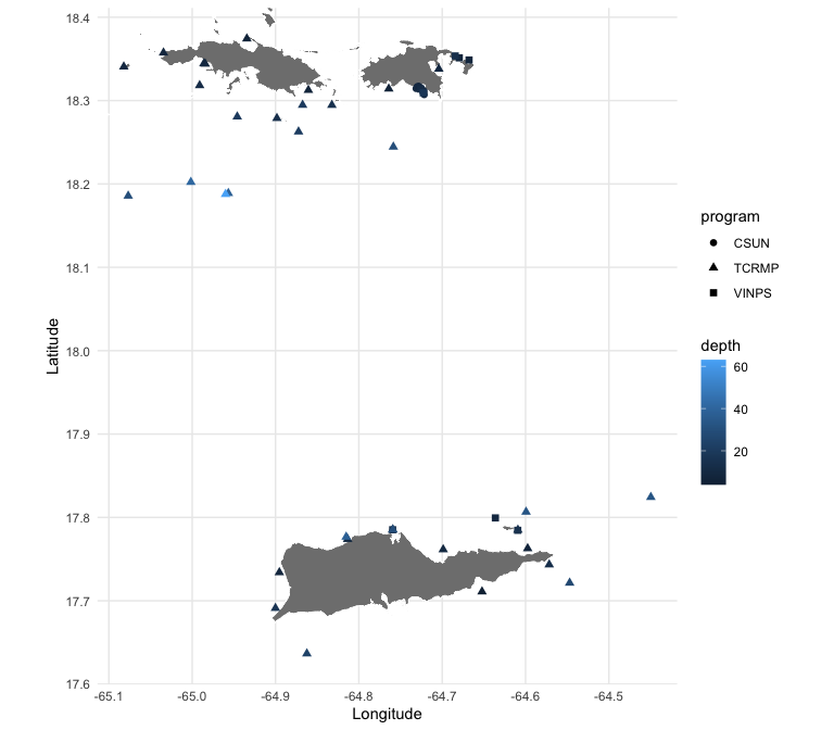
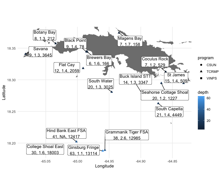
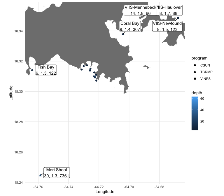
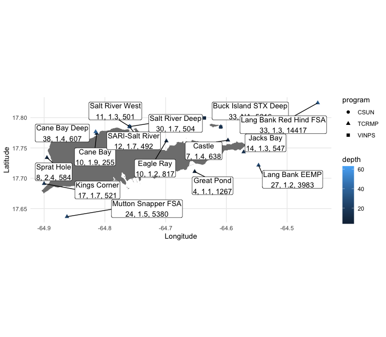
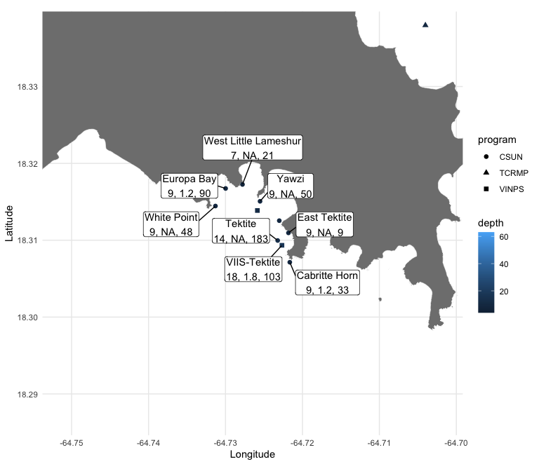
We build labeled static maps of the site network, split by island, for use in workshop activities. The sf, ggplot2, and ggrepel packages draw the island outlines, place the site points colored by depth, and label each site with its depth, rugosity, and distance from shore.
We read the site catalog into sitedat and load the USVI island shapefile as the map background.
Show code
sitedat <- dat
background_map <- st_read(dsn = "../shapefiles/pvishrpl/", layer = "pvishrpl", quiet = TRUE)
Show code
lon_range <- range(sitedat$lon)
lat_range <- range(sitedat$lat)

lon_rangestj <- range(sitedat |> filter(island=="STJ") |> select(lon))
lat_rangestj <- range(sitedat |> filter(island=="STJ") |> select(lat))

lon_rangestt <- range(sitedat |> filter(island=="STT") |> select(lon))
lat_rangestt <- range(sitedat |> filter(island=="STT") |> select(lat))

lon_rangestx <- range(sitedat |> filter(island=="STX") |> select(lon))
lat_rangestx <- range(sitedat |> filter(island=="STX") |> select(lat))

lon_rangestjcsun <- range(sitedat |> filter(program=="CSUN") |> select(lon))
lat_rangestjcsun <- range(sitedat |> filter(program=="CSUN") |> select(lat))
We define one overview map (pall) plus one labeled map per island group: St. Thomas (pstt), St. John (pstj), St. Croix (pstx), and the CSUN sites off St. John (pcsun).
Show code
pall <- ggplot() +
    geom_sf(data = background_map, fill = "grey50", color = "white") +

  geom_point(data = sitedat,
             aes(x = lon, y = lat, color = depth, shape = program),
             size = 2) +
  coord_sf(xlim = lon_range, ylim = lat_range) +
  labs(x = "Longitude", y = "Latitude") +
  theme_minimal()
  # guides(color = guide_legend(title = "deoth"))


pstt <- ggplot() +
    # Plot the background map
    geom_sf(data = background_map, fill = "grey50", color = "white") +

  geom_point(data = sitedat,
             aes(x = lon, y = lat, color = depth, shape = program),
             size = 2) +
  geom_label_repel(
    data = sitedat |> filter(island %in% c("STT")) ,
    aes(
      x = lon,
      y = lat,
      label = paste0(
        site,
        "\n",
        sprintf("%.0f", depth),
        ", ",
        sprintf("%.1f", rugosity),
        ", ",
        sprintf("%.0f", dist_from_shore)
        # "\nDist. from shore: ",
        # sprintf("%.2f", dist_from_shore)
      )
    ),
    box.padding = unit(0.5, "lines"),
    point.padding = unit(0, "lines"),
      label.padding = 0.1,
    segment.color = 'black'
  ) +
  coord_sf(xlim = lon_rangestt, ylim = lat_rangestt) +
  labs(x = "Longitude", y = "Latitude") +
  theme_minimal()
  # guides(color = guide_legend(title = "deoth"))

pstj <- ggplot() +
    # Plot the background map
    geom_sf(data = background_map, fill = "grey50", color = "white") +

  geom_point(data = sitedat,
             aes(x = lon, y = lat, color = depth, shape = program),
             size = 2) +
  geom_label_repel(
    data = sitedat |> filter(island %in% c("STJ") & program != "CSUN" & site != "VIIS_TK" & site != "VIIS-Yawzi" & site != "VIIS-Tektite") ,
    aes(
      x = lon,
      y = lat,
      label = paste0(
        site,
        "\n",
        sprintf("%.0f", depth),
        ", ",
        sprintf("%.1f", rugosity),
        ", ",
        sprintf("%.0f", dist_from_shore)
        # "\nDist. from shore: ",
        # sprintf("%.2f", dist_from_shore)
      )
    ),
    box.padding = unit(0.5, "lines"),
    point.padding = unit(0, "lines"),
      label.padding = 0.1,
    segment.color = 'black'
  ) +
  coord_sf(xlim = lon_rangestj, ylim = lat_rangestj) +
  labs(x = "Longitude", y = "Latitude") +
  theme_minimal()


pstx <- ggplot() +
    # Plot the background map
    geom_sf(data = background_map, fill = "grey50", color = "white") +

  geom_point(data = sitedat,
             aes(x = lon, y = lat, color = depth, shape = program),
             size = 2) +
  geom_label_repel(
    data = sitedat |> filter(island %in% c("STX")) ,
    aes(
      x = lon,
      y = lat,
      label = paste0(
        site,
        "\n",
        sprintf("%.0f", depth),
        ", ",
        sprintf("%.1f", rugosity),
        ", ",
        sprintf("%.0f", dist_from_shore)
      )
    ),
    box.padding = unit(0.5, "lines"),
    point.padding = unit(0, "lines"),
      label.padding = 0.1,
    segment.color = 'black'
  ) +
  coord_sf(xlim = lon_rangestx, ylim = lat_rangestx) +
  labs(x = "Longitude", y = "Latitude") +
  theme_minimal()

pcsun <- ggplot() +
    # Plot the background map
    geom_sf(data = background_map, fill = "grey50", color = "white") +

  geom_point(data = sitedat,
             aes(x = lon, y = lat, color = depth, shape = program),
             size = 2) +
  geom_label_repel(
    data = sitedat |> filter(program == "CSUN" | site == "VIIS-Yawzi" | site == "VIIS-Tektite"),
    aes(
      x = lon,
      y = lat,
      label = paste0(
        site,
        "\n",
        sprintf("%.0f", depth),
        ", ",
        sprintf("%.1f", rugosity),
        ", ",
        sprintf("%.0f", dist_from_shore)
      )
    ),
    box.padding = unit(0.5, "lines"),
    point.padding = unit(0, "lines"),
    label.padding = 0.1,
    segment.color = 'black'
  ) +
  coord_sf(xlim = lon_rangestjcsun+c(-0.02,0.02), ylim = lat_rangestjcsun+c(-0.02,0.02)) +
  labs(x = "Longitude", y = "Latitude") +
  theme_minimal()

library(patchwork)
#
# svg(filename="sitmap.svg", width = 15, height =15)
# pstt / pstj / pstx + plot_layout(guides= 'collect')
# dev.off()

# svg(filename="images/sitmapall.svg", width = 5, height =5)
# pall + theme(legend.position = "none") + scale_color_gradientn(colours = rainbow(10))
# dev.off()
#
# svg(filename="images/sitmapstt.svg", width = 15, height =9)
# pstt + theme(legend.position = "none")+ scale_color_gradientn(colours = rainbow(10))+ theme(panel.grid.major = element_blank(),
#                                                                                               panel.grid.minor = element_blank())
# dev.off()
#
# svg(filename="images/sitmapstx.svg", width = 15, height =8)
# pstx + theme(legend.position = "bottom")+ scale_color_gradientn(colours = rainbow(10)) + theme(panel.grid.major = element_blank(),
#                                                                                               panel.grid.minor = element_blank())
# dev.off()
#
# svg(filename="images/sitmapstj.svg", width = 15, height =8)
# pstj + theme(legend.position = "none")+ scale_color_gradientn(colours = rainbow(10))+ theme(panel.grid.major = element_blank(),
#                                                                                               panel.grid.minor = element_blank())
# dev.off()
#
# svg(filename="images/sitmapstjcsun.svg", width = 6, height =6)
# pcsun + theme(legend.position = "none")+ scale_color_gradientn(colours = rainbow(10))+ theme(panel.grid.major = element_blank(),
#                                                                                               panel.grid.minor = element_blank())
# dev.off()
The maps below show: an overview of all sites colored by depth, then the labeled per-island maps for St. Thomas, St. John, St. Croix, and the CSUN sites. Each site label reads depth, rugosity, and distance from shore.
Download the data
NoteDownload
The site master catalog and its metadata are available below.
version 1.0.0 • in-review • data ≤ 2023-12-31