Reef Code

about 2.1 Reformat raw benthic cover data 2.2 Cross-reference benthic codes 2.3 percentage cover of main benthic categories 2.4 percentage cover of coral genera 2.5 percentage cover of coral species 2.6 percentage cover of coral trait groups 2.7 percentage cover of algae taxa 2.8 percentage cover of sponge morphs 2.9 percentage cover of zoanthids and gorgonians 2.10 percentage cover of other benthic categories

internal drivers

3.1 coral health 3.2 coral interactions 3.3 fish biodiversity 3.3b fish biodiversity using NOAA data 3.4 herbivory 3.5 coral biodiversity 3.6 diadema 3.7 nuisance species

external drivers

4.1 site rugosity 4.2 site depth 4.3 site distances from shore 4.4 daily temperatures 4.5 monthly and annual DHW and temperature 4.6 currents 4.7 management 4.8 wave benthic orbital velocities pt 1 4.9 wave benthic orbital velocities pt 2 4.10 water quality 4.11 sedimentation 4.12 connectivity

resilience values

5.1 absolute and relative coral cover and diversity 5.2 resilience classification based on coral cover 5.3 benthic community: benthic organisms 5.4 NMDS of coral genera during recovery period

Reproductive Mode & RarityOlinger et al., In Review

Overview TCRMP VINPS CSUN Octocorals Interactive

2023, 2024 Bleaching EventOlinger et al. In Prep

VI Reef Resilience StudyOlinger et al. Coming Soon

(Any Others?)co-author suggestions welcome

3.3 Fish biodiversity

Last updated

July 6, 2026

3.3 Fish biodiversity

This page derives fish-community diversity metrics from the TCRMP annual fish transect counts and shows how each metric changed over time at every TCRMP site. The workflow reads the site master and the raw fish counts, reshapes the counts into a tidy long form, summarizes species richness and abundance per site and year, and computes Simpson’s diversity (1/D) per transect. The figures are site-faceted time series of species richness, abundance, both metrics split by trophic group, and Simpson’s diversity, each with a dashed reference line at the 2005 Caribbean-wide bleaching year. The page produces two derived data products, per-species counts and per-transect Simpson’s diversity, each with matching metadata.

Data sources

This page uses the raw TCRMP annual fish transect counts, joined to the RRS site master for site depth and ordering. Both come from the TCRMP program. The two derived products, per-species counts and per-transect Simpson’s diversity, are available in the Downloads section below.

Site data

The site master lists each monitoring site with its island, depth, and the year it was added.

Show code

sitedat <-
  read.csv(
    "../../../RRSdata/00_RRS_dataCatalogStatus/00_RRS_siteMaster_allSites_data.csv"
  )

Load fish counts

The raw TCRMP fish counts hold one row per species per transect, with abundance binned by size class.

Show code

fishcounts <-
  read.csv("../../../RRSdata/data_TCRMP/TCRMP_fishCounts_allSites_2003_2023_data.csv")

The block below defines an optional filter that keeps only annual surveys within the embargo window and only sites added no later than maxyearadded. It is inactive: all sites and years present in the raw file flow through to the summaries. See the science note in the report if the intended filter should be restored.

Show code

# sitekp <-
#   sitedat |>
#   filter(program == "TCRMP" &
#            yearadded <= maxyearadded) |>
#   select(site)
#
# fishcounts <-
#   fishcounts |>
#   filter(Period == "Annual") |>
#   filter(SampleYear >= minyear &
#            SampleYear <= maxyear) |>
#   filter(Location %in% sitekp$site)

The reformat drops the size-class bin columns and renames the remaining fields to short, tidy names, then removes the survey-period column.

Show code

fishcounts <- fishcounts |>
  select(-colnames(fishcounts[, 9:19]))

colnames(fishcounts) <- c(
  "site",
  "year",
  "month",
  "period",
  "transect",
  "sppname",
  "commonname",
  "trophicgroup",
  "counts"
)

fishcounts <- fishcounts |> select(-period)

The tidied counts cover 35 sites and survey years 2003 to 2022.

Summarize for plotting

What happens here: the counts are summarized two ways. First per trophic group (richness and abundance per transect, then averaged across transects with a standard deviation), and second across all species (total richness and abundance per transect, then averaged with a standard deviation). These summaries feed the time-series figures below.

Show code

fishsum_troph <- fishcounts |>
  group_by(year, site, transect, trophicgroup) |>
  summarise(diversity = length(unique(sppname)),
            counts = sum(counts))

fishsum_trophsum <- fishsum_troph |>
  group_by(year, site, trophicgroup) |>
  summarise(
    meandiv = mean(diversity),
    sddiv = sd(diversity),
    meancounts = mean(counts),
    sdcounts = sd(counts)
  )

fishsum_tot <- fishcounts |>
  group_by(year, site, transect) |>
  summarise(diversity = length(unique(sppname)),
            counts = sum(counts))

fishsum_totsum <- fishsum_tot |>
  group_by(year, site) |>
  summarise(
    meandiv = mean(diversity),
    sddiv = sd(diversity),
    meancounts = mean(counts),
    sdcounts = sd(counts)
  )

Figure 1 shows annual mean species richness at each TCRMP site, with sites ordered shallow to deep and the ribbon showing the standard deviation across transects. The dashed line marks the 2005 bleaching year.

Show code

fishsum_totsum <-
  merge(fishsum_totsum, sitedat, by = "site")
fishsum_totsum <-
  fishsum_totsum[order(fishsum_totsum$depth),]

fishsum_totsum$site <- factor(fishsum_totsum$site,
                              levels = unique(fishsum_totsum$site))

ggplot(
  fishsum_totsum,
  aes(
    x = year,
    y = meandiv,
    fill = depth,
    ymin = meandiv - sddiv,
    ymax = meandiv + sddiv
  )
) +
  scale_fill_continuous(low = "red", high = "blue") +
  facet_wrap(. ~ site , scales = "fixed") +
  geom_ribbon(alpha = .5) +
  geom_line(size = 0.25) +
  geom_point(size = 0.5) +
  ylab("species richness") +
  # coord_cartesian(ylim = c(0,1))+
  # scale_y_continuous(expand = c(0, 0)) +
  geom_vline(
    xintercept = 2005,
    color = "gray50",
    alpha = 0.5,
    lty = "dashed"
  ) +
  theme_bw() +
  theme(strip.text = element_text(size = 10)) +
  theme(legend.position = "bottom") +
  theme(panel.grid.major = element_blank(),
        panel.grid.minor = element_blank())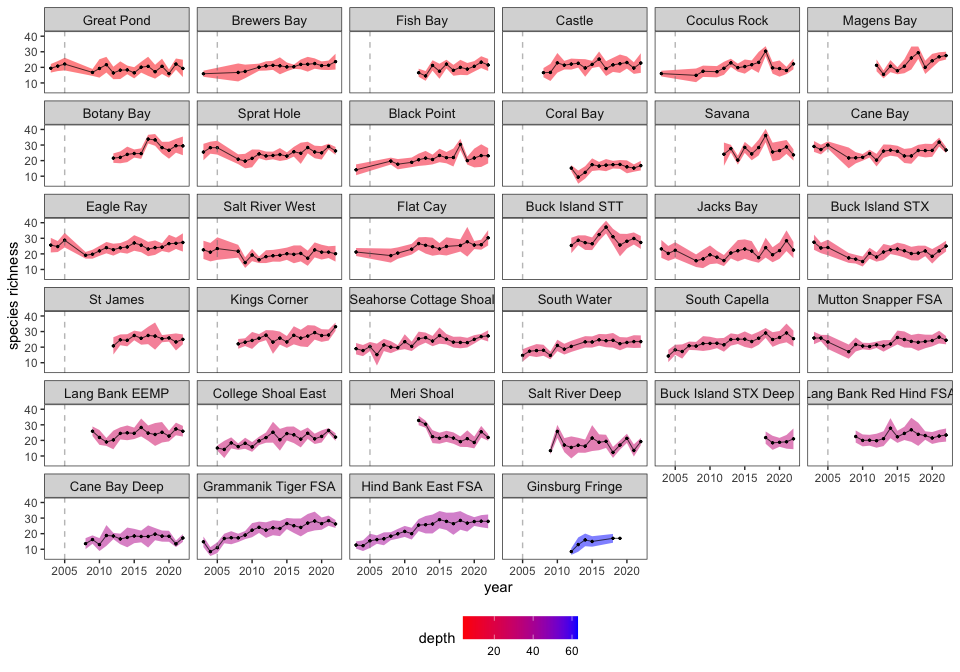

Sec 3.3 Figure 1: Annual mean fish species richness across TCRMP sites, faceted by site and ordered shallow to deep. The ribbon shows plus or minus one standard deviation across transects. The dashed line marks the 2005 bleaching year.

Figure 2 shows annual mean fish abundance (total individuals) at each site, ordered shallow to deep, with the standard-deviation ribbon and the 2005 reference line.

Show code

ggplot(
  fishsum_totsum,
  aes(
    x = year,
    y = meancounts,
    fill = depth,
    ymin = meancounts - sdcounts,
    ymax = meancounts + sdcounts
  )
) +
  scale_fill_continuous(low = "red", high = "blue") +
  facet_wrap(. ~ site , scales = "fixed") +
  geom_ribbon(alpha = .5) +
  geom_line(size = 0.25) +
  geom_point(size = 0.5) +
  ylab("abundance (# individuals)") +
  # coord_cartesian(ylim = c(0,1))+
  # scale_y_continuous(expand = c(0, 0)) +
  geom_vline(
    xintercept = 2005,
    color = "gray50",
    alpha = 0.5,
    lty = "dashed"
  ) +
  theme_bw() +
  theme(strip.text = element_text(size = 10)) +
  theme(legend.position = "bottom") +
  theme(panel.grid.major = element_blank(),
        panel.grid.minor = element_blank())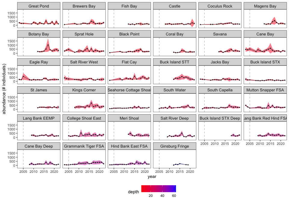

Sec 3.3 Figure 2: Annual mean fish abundance (individuals) across TCRMP sites, faceted by site and ordered shallow to deep. The ribbon shows plus or minus one standard deviation across transects. The dashed line marks the 2005 bleaching year.

Figure 3 splits annual mean species richness by trophic group, so each site facet shows one colored series per group. The standard-deviation ribbon and the 2005 reference line carry over.

Show code

fishsum_trophsum <-
  merge(fishsum_trophsum, sitedat, by = "site")
fishsum_trophsum <-
  fishsum_trophsum[order(fishsum_trophsum$depth),]
fishsum_trophsum$site <- factor(fishsum_trophsum$site,
                                levels = unique(fishsum_trophsum$site))

ggplot(
  fishsum_trophsum,
  aes(
    x = year,
    y = meandiv,
    color = trophicgroup,
    fill = trophicgroup,
    ymin = meandiv - sddiv,
    ymax = meandiv + sddiv
  )
) +
  facet_wrap(. ~ site , scales = "fixed") +
  geom_ribbon(alpha = 0.25, linewidth = 0) +
  geom_line(size = 0.25) +
  geom_point(size = 0.5) +
  ylab("species richness") +
  # coord_cartesian(ylim = c(0,1))+
  # scale_y_continuous(expand = c(0, 0)) +
  geom_vline(
    xintercept = 2005,
    color = "gray50",
    alpha = 0.5,
    lty = "dashed"
  ) +
  theme_bw() +
  theme(strip.text = element_text(size = 10)) +
  theme(legend.position = "bottom") +
  theme(panel.grid.major = element_blank(),
        panel.grid.minor = element_blank())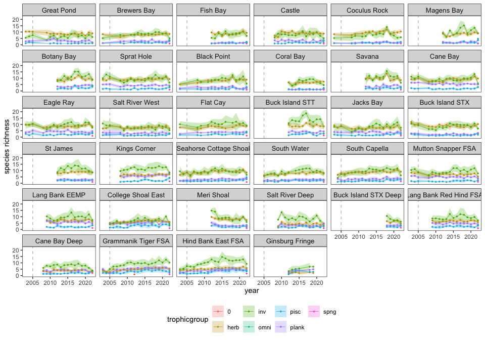

Sec 3.3 Figure 3: Annual mean fish species richness across TCRMP sites split by trophic group, faceted by site and ordered shallow to deep. The ribbon shows plus or minus one standard deviation across transects. The dashed line marks the 2005 bleaching year.

Figure 4 splits annual mean abundance by trophic group. The abundance axis is capped at 800 individuals so the between-site pattern stays readable.

Show code

ggplot(
  fishsum_trophsum,
  aes(
    x = year,
    y = meancounts,
    color = trophicgroup,
    fill = trophicgroup,
    ymin = meancounts - sdcounts,
    ymax = meancounts + sdcounts
  )
) +
  facet_wrap(. ~ site , scales = "fixed") +
  geom_ribbon(alpha = 0.25, linewidth = 0) +
  geom_line(size = 0.25) +
  geom_point(size = 0.5) +
  ylab("abundance (# individuals)") +
  coord_cartesian(ylim = c(0, 800)) +
  # scale_y_continuous(expand = c(0, 0)) +
  geom_vline(
    xintercept = 2005,
    color = "gray50",
    alpha = 0.5,
    lty = "dashed"
  ) +
  theme_bw() +
  theme(strip.text = element_text(size = 10)) +
  theme(legend.position = "bottom") +
  theme(panel.grid.major = element_blank(),
        panel.grid.minor = element_blank())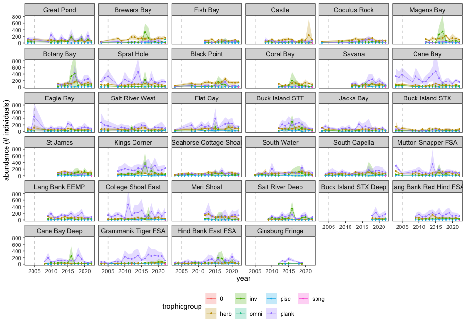

Sec 3.3 Figure 4: Annual mean fish abundance (individuals) across TCRMP sites split by trophic group, faceted by site and ordered shallow to deep. The abundance axis is capped at 800. The ribbon shows plus or minus one standard deviation across transects. The dashed line marks the 2005 bleaching year.

Simpson’s diversity

Simpson’s index considers both species richness and evenness, like the Shannon-Wiener index. It is defined as

\[ D = \sum_{i=1}^{S} p_i^2 \]

where \(p_i\) is the proportion of individuals of species \(i\) and \(S\) is the number of species. A higher \(D\) indicates lower diversity, so this page reports the reciprocal \(1/D\), which increases with diversity.

What happens here: the code computes \(1/D\) per site, year, month, and transect, then averages it across transects with a standard deviation for each site and year.

Show code

simpson_calculation <- fishcounts |>
  group_by(site, year, month, transect) |>
  summarise(total = sum(counts))  |>
  left_join(fishcounts)  |>
  mutate(proportion = counts / total) |>
  group_by(site, year, month, transect)  |>
  summarise(simpson_index = sum(proportion ^ 2))  |>
  mutate(simpson_diversity = 1 / simpson_index)

simpson_calculation_sum <- simpson_calculation |>
  group_by(site, year) |>
  summarise(meandiv = mean(simpson_diversity),
            sddiv = sd(simpson_diversity))

Figure 5 shows annual mean Simpson’s diversity (1/D) at each site, ordered shallow to deep, with the standard-deviation ribbon and the 2005 reference line.

Show code

simpson_calculation_sum <-
  merge(simpson_calculation_sum, sitedat, by = "site")
simpson_calculation_sum <-
  simpson_calculation_sum[order(simpson_calculation_sum$depth),]

simpson_calculation_sum$site <- factor(simpson_calculation_sum$site,
                                       levels = unique(simpson_calculation_sum$site))

p <-
  ggplot(
    simpson_calculation_sum,
    aes(
      x = year,
      y = meandiv,
      fill = depth,
      ymin = meandiv - sddiv,
      ymax = meandiv + sddiv
    )
  ) +
  scale_fill_continuous(low = "red", high = "blue") +
  facet_wrap(. ~ site , scales = "fixed") +
  geom_ribbon(alpha = .5) +
  geom_line(size = 0.25) +
  geom_point(size = 0.5) +
  ylab("Simpsons diversity (1/D)") +
  # coord_cartesian(ylim = c(0,1))+
  # scale_y_continuous(expand = c(0, 0)) +
  geom_vline(
    xintercept = 2005,
    color = "gray50",
    alpha = 0.5,
    lty = "dashed"
  ) +
  theme_bw() +
  theme(strip.text = element_text(size = 10)) +
  theme(legend.position = "bottom") +
  theme(panel.grid.major = element_blank(),
        panel.grid.minor = element_blank())

p

# svg(filename="fishdiv.svg", width = 13, height =13)
# p
# dev.off()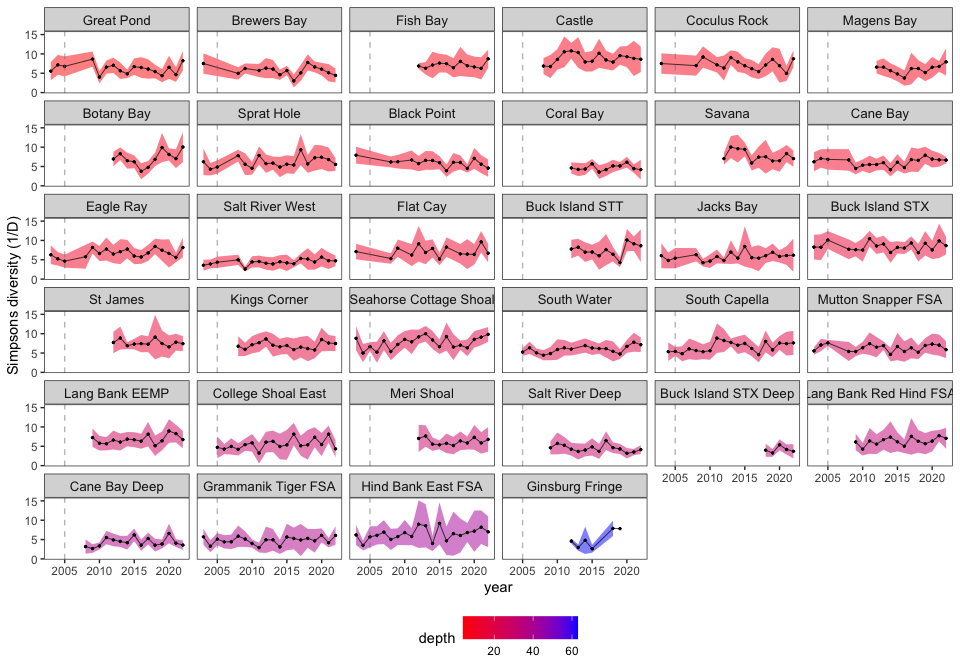

Sec 3.3 Figure 5: Annual mean Simpson’s diversity (1/D) across TCRMP sites, faceted by site and ordered shallow to deep. The ribbon shows plus or minus one standard deviation across transects. The dashed line marks the 2005 bleaching year.

Downloads

Each data product below downloads with its matching metadata file.

version 1.0.0 • in-review • data ≤ 2023-12-31

3.3 Fish biodiversity

On this page

Data sources

Site data

Load fish counts

Summarize for plotting

Simpson’s diversity

Downloads