Show code
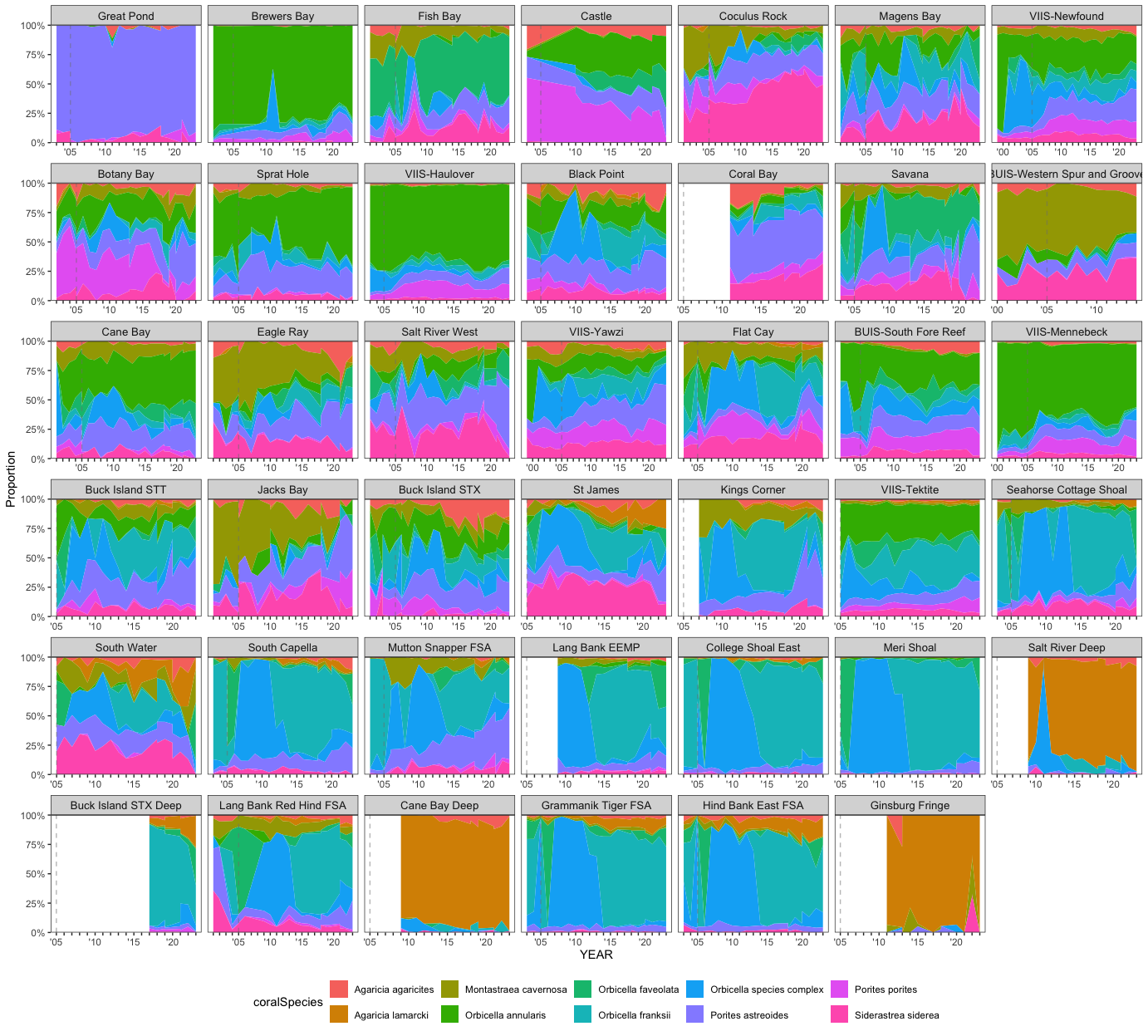
load("benthicCoverXrefBenthicCodes.RData")This page aggregates surveyed benthic points to the coral-species level and calculates annual percent cover of each species at every monitoring site. It reads the reformatted survey data and the corrected benthic-code cross-reference produced by parts 1 and 2 of the benthic pipeline, groups points by species, and averages cover per site and year. The two figures show cover over time: Figure 1 stacks every species by site (shallow to deep), and Figure 2 shows the proportional make-up of the ten highest-cover species. The page writes the site-by-year coral-species cover product (s2pt5_benthicCoverCoralSpecies) that downstream publication and resilience pages read.
This is a multi-program page. TCRMP and VINPS have transect replicates, so their site means carry standard error. CSUN has no transect replicate at the site level, so its cover is computed cumulatively and shows no error bar. The programs also start in different years (VINPS around 1999, CSUN in 1992), so the site panels do not all begin at the same point on the x-axis.
This page reads the reformatted survey data and corrected benthic-code cross-reference (benthicCoverXrefBenthicCodes.RData) written by parts 1 and 2 of the benthic pipeline (sections 2.1 and 2.2), which combine the TCRMP, VINPS, and CSUN programs. The cross-reference carries the UAGA correction that restores VINPS Agaricia agaricites, and the date range respects the site embargo (data through 2023). The derived site-by-year coral-species cover product this page computes is available in the Downloads section below.
We load the reformatted survey data and cross-referenced benthic codes written by parts 1 and 2 of the pipeline (sections 2.1 and 2.2).
load("benthicCoverXrefBenthicCodes.RData")We set groupingvar to coralSpecies so the pipeline groups taxa at the species level on this page, and section to s2pt5 for output naming.
groupingvar <- "coralSpecies"
section <- "s2pt5" # for namingbenthicDat into coral speciesWe restrict benthicCodes to the coral category so the grouping covers coral species only.
The include below runs the shared cross-referencing pipeline (_middlexref.qmd). It maps each program’s benthic-code columns to coral species, merges TCRMP, VINPS, and CSUN into one long table, and produces groupedBenthicDat, the per-record coral-species cover table used for the rest of the page. The UAGA guard in that include warns if any data column carries a taxon code missing from the cross-reference.
getBenthicDatColInds()this is one of two functions that connect benthicDat to benthicCodes for all three programs.
getBenthicDatColInds() makes _columnInds that stores column indices of benthic codes corresponding to each item of coralSpecies arguments:
benthicDat is benthic dataset of interest
codecolumn is the name of the column of benthic code containing the code for benthicdat
groupingcolumn is the name of the column of benthic codes where the grouping variable of interest is stored.
getBenthicDatColInds <-
  function(benthicDat, codecolumn, groupingcolumn) {
    codecolind <-
      which(colnames(benthicCodes) == codecolumn)
    groupingcolind <-
      which(colnames(benthicCodes) == groupingcolumn)
    genusdf <-
      data.frame(group =
                   unique(benthicCodes[, groupingcolind]),
                 colinds =
                   rep(0, length(unique(benthicCodes[, groupingcolind]))))
    for (i in 1:nrow(genusdf)) {
      codei <-
        benthicCodes[which(benthicCodes[, groupingcolind] == genusdf$group[i]), ]
      genusdf$colinds[i] <-
        list(which(colnames(benthicDat) %in% codei[, codecolind]))
    }
    # UAGA-guard: warn on benthicDat data columns whose code is absent from benthicCodes and is
    # therefore silently dropped (the footgun that lost VINPS Agaricia agaricites, code UAGA).
    .known <- benthicCodes[[codecolind]]; .known <- .known[nchar(.known) > 0]
    .meta_cols <- c("program","date","site","period","replicate","replicatetype","nopts",
                    "Year","Date","SiteFullName","year","month","percentCover_allCoral",
                    "PC","Check","Notes","Transect")
    .dropped <- setdiff(colnames(benthicDat), c(.known, .meta_cols))
    if (length(.dropped) > 0)
      warning("getBenthicDatColInds(", codecolumn, "): ", length(.dropped),
              " data column(s) have codes absent from benthicCodes and are DROPPED: ",
              paste(.dropped, collapse = ", "), " -- add them to benthicCodes if they are taxa.")
    return(genusdf)
  }
apply getBenthicDatColInds() to _benthicDat dataframes . preview tcrmp_columnInds
tcrmp_columnInds <-
  getBenthicDatColInds(tcrmp_benthicDat, "tcrmp_Code", "tcrmp_Meaning")
vinps_columnInds <-
  getBenthicDatColInds(vinps_benthicDat, "vinps_TaxonCode", "tcrmp_Meaning")

kbl(tcrmp_columnInds) |>
  kable_paper(full_width = F) |>
  kable_styling(
    fixed_thead = T,
    bootstrap_options = c("hover", "condensed"),
    font_size = 8
  ) |>
scroll_box(width = "100%", height = "250px")| group | colinds |
|---|---|
| Millepora alcicornis | 38 |
| Millepora complanata | 39 |
| Millepora squarrosa | 40 |
| Dendrogyra cylindrus | 22 |
| Acropora cervicornis | 9 |
| Acropora palmata | 15 |
| Acropora prolifera | 16 |
| Orbicella faveolata | 48 |
| Orbicella franksii | 49 |
| Orbicella species complex | 50 |
| Scolymia lacera | 65 |
| Scolymia cubensis | 61 |
| Scolymia spp. | 62 |
| Porites branneri | 52 |
| Mycetophyllia aliciae | 31 |
| Mycetophyllia daniana | 36 |
| Mycetophyllia lamarckiana | 41 |
| Mycetophyllia spp. | 45 |
| Mussa angulosa | 32 |
| Madracis mirabilis | 42 |
| Isopyhyllastrea rigida | 28 |
| Coral spp. | 20 |
| Juvenile coral spp. | 21 |
| Helioseris cucullata | 27 |
| Oculina diffusa | 47 |
| Solenastrea bournoni | 60 |
| Solenastrea hyades | 63 |
| Tubastraea coccinea | 69 |
| Stephanocoenia intercepta | 64 |
| Siderastrea spp. | 68 |
| Siderastrea siderea | 67 |
| Orbicella annularis | 46 |
| Montastraea cavernosa | 34 |
| Montastraea spp. | 44 |
| Meandrina meandrites | 43 |
| Favia fragum | 26 |
| Eusmilia fastigiata | 25 |
| Diploria labyrinthiformis | 23 |
| Dichocoenia stokesii | 24 |
| Colpophyllia natans | 19 |
| Pseudodiploria clivosa | 55 |
| Pseudodiploria strigosa | 59 |
| Siderastrea radians | 66 |
| Porites divaricata | 56 |
| Porites astreoides | 51 |
| Porites furcata | 57 |
| Branching Porites spp. | 53 |
| Porites porites | 58 |
| Mycetophyllia ferox | 37 |
| Manicina areolata | 33 |
| Madracis decactis | 35 |
| Madracis formosa | 30 |
| Agaricia fragilis | 10 |
| Agaricia agaricites | 8 |
| Agaricia grahamae | 11 |
| Agaricia humilis | 13 |
| Agaricia spp. | 12 |
| Agaricia tenuifolia | 17 |
| Agaricia undata | 18 |
| Agaricia lamarcki | 14 |
| Isophyllia sinuosa | 29 |
makeGroupedBenthicDat()this is the second function that connects benthicDat to benthicCodes for all three programs.
makeGroupedBenthicDat() extracts the column indices (colinds) from each row of *_columnInds.
If only one index in colinds , assigns the corresponding column from benthicdat to the i-th column of a data frame _groupedBenthicDat.
if more than one index in colinds, stores row sum of benthicDat[,colinds] in the i-th column of _groupedBenthicDat.
arguments:
benthicDat is benthic dataset of interest
columnInds is the output of getBenthicDatColInds() above that contains column indices of benthic codes for each benthic subgroup of interest
makeGroupedBenthicDat <- function(benthicDat, columnInds) {
  groupeddat <- data.frame(matrix(nrow = nrow(benthicDat),
                                  ncol = nrow(columnInds)))
  colnames(groupeddat) <- columnInds$group
   benthicDat <- benthicDat %>% dplyr::mutate(dplyr::across(dplyr::where(is.numeric), ~replace(.x, is.na(.x), 0)))
  for (i in 1:nrow(columnInds)) {
    geni <- columnInds[i,]
    datcoli <- unlist(geni$colinds)
    if (length(datcoli) == 1) {
      groupeddat[, i] <- benthicDat[, datcoli]
    } else {
      groupeddat[, i] <- rowSums(benthicDat[, datcoli])
    }
  }
  groupeddat <- cbind(benthicDat[, 1:6], groupeddat)
  return(groupeddat)
}
apply makeGroupedBenthicDat() to _benthicDat and _columnInds . preview tcrmp_groupedBenthicDat.
tcrmp_groupedBenthicDat <-
  makeGroupedBenthicDat(tcrmp_benthicDat, tcrmp_columnInds)
vinps_groupedBenthicDat <-
  makeGroupedBenthicDat(vinps_benthicDat, vinps_columnInds)

kbl(head(tcrmp_groupedBenthicDat)) |>
  kable_paper(full_width = F) |>
  kable_styling(
    fixed_thead = T,
    bootstrap_options = c("hover", "condensed"),
    font_size = 8
  ) |>
scroll_box(width = "100%", height = "250px")| program | date | site | period | replicate | replicatetype | Millepora alcicornis | Millepora complanata | Millepora squarrosa | Dendrogyra cylindrus | Acropora cervicornis | Acropora palmata | Acropora prolifera | Orbicella faveolata | Orbicella franksii | Orbicella species complex | Scolymia lacera | Scolymia cubensis | Scolymia spp. | Porites branneri | Mycetophyllia aliciae | Mycetophyllia daniana | Mycetophyllia lamarckiana | Mycetophyllia spp. | Mussa angulosa | Madracis mirabilis | Isopyhyllastrea rigida | Coral spp. | Juvenile coral spp. | Helioseris cucullata | Oculina diffusa | Solenastrea bournoni | Solenastrea hyades | Tubastraea coccinea | Stephanocoenia intercepta | Siderastrea spp. | Siderastrea siderea | Orbicella annularis | Montastraea cavernosa | Montastraea spp. | Meandrina meandrites | Favia fragum | Eusmilia fastigiata | Diploria labyrinthiformis | Dichocoenia stokesii | Colpophyllia natans | Pseudodiploria clivosa | Pseudodiploria strigosa | Siderastrea radians | Porites divaricata | Porites astreoides | Porites furcata | Branching Porites spp. | Porites porites | Mycetophyllia ferox | Manicina areolata | Madracis decactis | Madracis formosa | Agaricia fragilis | Agaricia agaricites | Agaricia grahamae | Agaricia humilis | Agaricia spp. | Agaricia tenuifolia | Agaricia undata | Agaricia lamarcki | Isophyllia sinuosa |
|---|---|---|---|---|---|---|---|---|---|---|---|---|---|---|---|---|---|---|---|---|---|---|---|---|---|---|---|---|---|---|---|---|---|---|---|---|---|---|---|---|---|---|---|---|---|---|---|---|---|---|---|---|---|---|---|---|---|---|---|---|---|---|---|---|---|---|
| TCRMP | 2001-04-25 | Cane Bay | Annual | 1 | transect | 0.00 | 0 | 0 | 0 | 0 | 0 | 0 | 0 | 0 | 1.15 | 0 | 0 | 0 | 0 | 0.00 | 0 | 0 | 0 | 0 | 0 | 0 | 0.00 | 0 | 0 | 0 | 0 | 0 | 0 | 0.00 | 0 | 0.00 | 0 | 1.53 | 0 | 0 | 0 | 0 | 0.00 | 0 | 0.00 | 0 | 0.00 | 0 | 0.00 | 2.30 | 0 | 0 | 0.00 | 0.00 | 0 | 0 | 0 | 0 | 0.00 | 0 | 0 | 0 | 0 | 0 | 0 | 0.00 |
| TCRMP | 2001-04-25 | Cane Bay | Annual | 2 | transect | 0.00 | 0 | 0 | 0 | 0 | 0 | 0 | 0 | 0 | 12.11 | 0 | 0 | 0 | 0 | 0.00 | 0 | 0 | 0 | 0 | 0 | 0 | 0.78 | 0 | 0 | 0 | 0 | 0 | 0 | 0.00 | 0 | 0.00 | 0 | 5.86 | 0 | 0 | 0 | 0 | 2.34 | 0 | 0.39 | 0 | 0.00 | 0 | 0.00 | 2.73 | 0 | 0 | 1.56 | 0.00 | 0 | 0 | 0 | 0 | 1.17 | 0 | 0 | 0 | 0 | 0 | 0 | 0.00 |
| TCRMP | 2001-04-25 | Cane Bay | Annual | 3 | transect | 0.00 | 0 | 0 | 0 | 0 | 0 | 0 | 0 | 0 | 22.09 | 0 | 0 | 0 | 0 | 0.39 | 0 | 0 | 0 | 0 | 0 | 0 | 0.78 | 0 | 0 | 0 | 0 | 0 | 0 | 0.00 | 0 | 1.94 | 0 | 2.71 | 0 | 0 | 0 | 0 | 0.00 | 0 | 0.78 | 0 | 0.39 | 0 | 0.78 | 2.33 | 0 | 0 | 3.10 | 0.00 | 0 | 0 | 0 | 0 | 1.55 | 0 | 0 | 0 | 0 | 0 | 0 | 0.39 |
| TCRMP | 2001-04-25 | Cane Bay | Annual | 4 | transect | 0.00 | 0 | 0 | 0 | 0 | 0 | 0 | 0 | 0 | 21.38 | 0 | 0 | 0 | 0 | 0.00 | 0 | 0 | 0 | 0 | 0 | 0 | 0.36 | 0 | 0 | 0 | 0 | 0 | 0 | 0.00 | 0 | 0.00 | 0 | 5.07 | 0 | 0 | 0 | 0 | 0.00 | 0 | 0.00 | 0 | 0.00 | 0 | 0.00 | 1.45 | 0 | 0 | 0.36 | 1.45 | 0 | 0 | 0 | 0 | 0.72 | 0 | 0 | 0 | 0 | 0 | 0 | 0.00 |
| TCRMP | 2001-04-25 | Cane Bay | Annual | 5 | transect | 0.00 | 0 | 0 | 0 | 0 | 0 | 0 | 0 | 0 | 17.72 | 0 | 0 | 0 | 0 | 0.00 | 0 | 0 | 0 | 0 | 0 | 0 | 0.39 | 0 | 0 | 0 | 0 | 0 | 0 | 0.00 | 0 | 3.54 | 0 | 0.00 | 0 | 0 | 0 | 0 | 0.00 | 0 | 0.00 | 0 | 0.00 | 0 | 0.00 | 0.39 | 0 | 0 | 0.00 | 0.00 | 0 | 0 | 0 | 0 | 1.18 | 0 | 0 | 0 | 0 | 0 | 0 | 0.00 |
| TCRMP | 2001-04-25 | Cane Bay | Annual | 6 | transect | 0.38 | 0 | 0 | 0 | 0 | 0 | 0 | 0 | 0 | 9.02 | 0 | 0 | 0 | 0 | 0.00 | 0 | 0 | 0 | 0 | 0 | 0 | 0.38 | 0 | 0 | 0 | 0 | 0 | 0 | 0.38 | 0 | 0.38 | 0 | 1.13 | 0 | 0 | 0 | 0 | 0.00 | 0 | 0.00 | 0 | 0.38 | 0 | 0.00 | 1.88 | 0 | 0 | 2.26 | 0.38 | 0 | 0 | 0 | 0 | 0.38 | 0 | 0 | 0 | 0 | 0 | 0 | 0.00 |
benthicDat from three programsnow have three _groupedBenthicDat, need to merge them, start by comparing the column names, because some are missing from csun.
make sure each _groupedBenthicDat has the same column names
for (col in missing_columns_tcrmp) {
  tcrmp_groupedBenthicDat[[col]] <- NA
}
for (col in missing_columns_vinps) {
  vinps_groupedBenthicDat[[col]] <- NA
}tcrmp_groupedBenthicDat <- tcrmp_groupedBenthicDat[, all_columns]
vinps_groupedBenthicDat <- vinps_groupedBenthicDat[, all_columns]groupedBenthicDat.groupedBenthicDat <-
rbind(tcrmp_groupedBenthicDat,
vinps_groupedBenthicDat)groupedBenthicDat into long format.For TCRMP and VINPS we calculate annual transect-averaged percent cover of coral species at each site, so the site means carry standard error from the transect replicates. For CSUN we calculate cumulative percent cover at each site because CSUN has no transect replicate.
We sum cover across species within each replicate, then average across replicates to get total coral cover per site and year with its standard error.
totaldatCovSum <- groupedBenthicDat |>
  dplyr::group_by(year, date, program, site, period, replicate) |>
  dplyr::summarise(perccover = sum(perccover))

totaldatCovSum <- totaldatCovSum |>
  dplyr::group_by(year, date, program, site) |>
  dplyr::summarise(
    meancov = mean(perccover),
    sdcov = sd(perccover),
    secov = sd(perccover) / (sqrt(length(perccover))),
    n = length(perccover)
  )

totaldatCovSum <- totaldatCovSum %>% dplyr::mutate(dplyr::across(dplyr::where(is.numeric), ~replace(.x, is.na(.x), 0)))We average cover per species across replicates to get species-level cover per site and year.
groupedBenthicDatCovSum <- groupedBenthicDat |>
  dplyr::group_by(year, date, program, site, period, coralSpecies) |>
  dplyr::summarise(
    meancov = mean(perccover),
    sdcov = sd(perccover),
    secov = sd(perccover) / (sqrt(length(perccover))),
    n = length(perccover)
  )
groupedBenthicDatCovSum <- groupedBenthicDatCovSum %>% dplyr::mutate(dplyr::across(dplyr::where(is.numeric), ~replace(.x, is.na(.x), 0)))We add site depth and order the sites shallow to deep so the facets read in depth order.
#add site info so can plot according to increasing depth
groupedBenthicDatCovSum <-
  merge(groupedBenthicDatCovSum, sitedat, by = "site")
groupedBenthicDatCovSum <-
  groupedBenthicDatCovSum[order(groupedBenthicDatCovSum$depth), ]
groupedBenthicDatCovSum$site <- factor(groupedBenthicDatCovSum$site,
                                       levels = unique(groupedBenthicDatCovSum$site))

#add site info so can plot according to increasing depth
totaldatCovSum <-
  merge(totaldatCovSum, sitedat, by = "site")
totaldatCovSum <-
  totaldatCovSum[order(totaldatCovSum$depth), ]
totaldatCovSum$site <- factor(totaldatCovSum$site,
                              levels = unique(totaldatCovSum$site))
create_stacked_area_plot() builds the site-faceted stacked-area figure: each site panel stacks species cover over time, overlays total coral cover as black points with standard-error linerange, and marks the 2005 bleaching year with a dashed line.
create_stacked_area_plot <- function(data_stacked,
                                     data_total,
                                     x_var = "year",
                                     y_var = "meancov",
                                     fill_var = "coralSpecies",
                                     facet_var = "site",
                                     error_var = "secov",
                                     min_year = NULL,
                                     max_year = NULL,
                                     highlight_year = NULL,
                                     max_facets_per_page = 35) {
  # Determine x-axis limits if not provided
  if (is.null(min_year))
    min_year <- floor(min(data_stacked[[x_var]]))
  if (is.null(max_year))
    max_year <- ceiling(max(data_stacked[[x_var]]))

  # Calculate optimal number of rows and columns
  n_facets <- length(unique(data_stacked[[facet_var]]))
  n_facets <- min(n_facets, max_facets_per_page)  # Limit to max_facets_per_page
  n_col <- ceiling(sqrt(n_facets))
  n_row <- ceiling(n_facets / n_col)

  # Create base plot
  p <- ggplot() +
    geom_area(data = data_stacked,
              aes(x = .data[[x_var]], y = .data[[y_var]], fill = .data[[fill_var]]),
              position = 'stack') +
    geom_point(
      data = data_total,
      aes(x = .data[[x_var]], y = .data[[y_var]]),
      color = "black",
      size = 0.5
    ) +
    geom_linerange(
      data = data_total,
      aes(
        x = .data[[x_var]],
        ymin = .data[[y_var]] - .data[[error_var]],
        ymax = .data[[y_var]] + .data[[error_var]]
      ),
      color = "black",
      linewidth = 0.5
    ) +
    facet_wrap(vars(.data[[facet_var]]), nrow = n_row, ncol = n_col, scales = "free_x") +
    labs(y = "Percent cover", x = toupper(x_var)) +
    scale_y_continuous(expand = c(0, 0)) +
    scale_x_continuous(
      expand = expansion(mult = 0.04),
      breaks = seq(min_year, max_year, by = 1),
      labels = function(x)
        ifelse(x %% 5 == 0, paste0("'", substr(x, 3, 4)), "")
    ) +
    theme_bw() +
    theme(
      strip.text = element_text(size = 10),
      legend.position = "bottom",
      panel.grid = element_blank()
    )

  # Add highlight line if specified
  if (!is.null(highlight_year)) {
    p <- p + geom_vline(
      xintercept = highlight_year,
      color = "gray50",
      alpha = 0.5,
      linetype = "dashed"
    )
  }

  return(p)
}
Figure 1 shows total coral cover falling at most sites after the 2005 bleaching year, with the species make-up of that cover visible in each panel. Sites read shallow to deep, and TCRMP and VINPS panels carry standard-error lineranges while CSUN panels do not.
# Usage:
stack <- create_stacked_area_plot(
  data_stacked = groupedBenthicDatCovSum,
  data_total = totaldatCovSum,
  min_year = minyear,
  max_year = maxyear,
  highlight_year = 2005,
  fill_var = "coralSpecies",
  max_facets_per_page = length(unique(groupedBenthicDatCovSum$site))
)

# Display the plot
print(stack)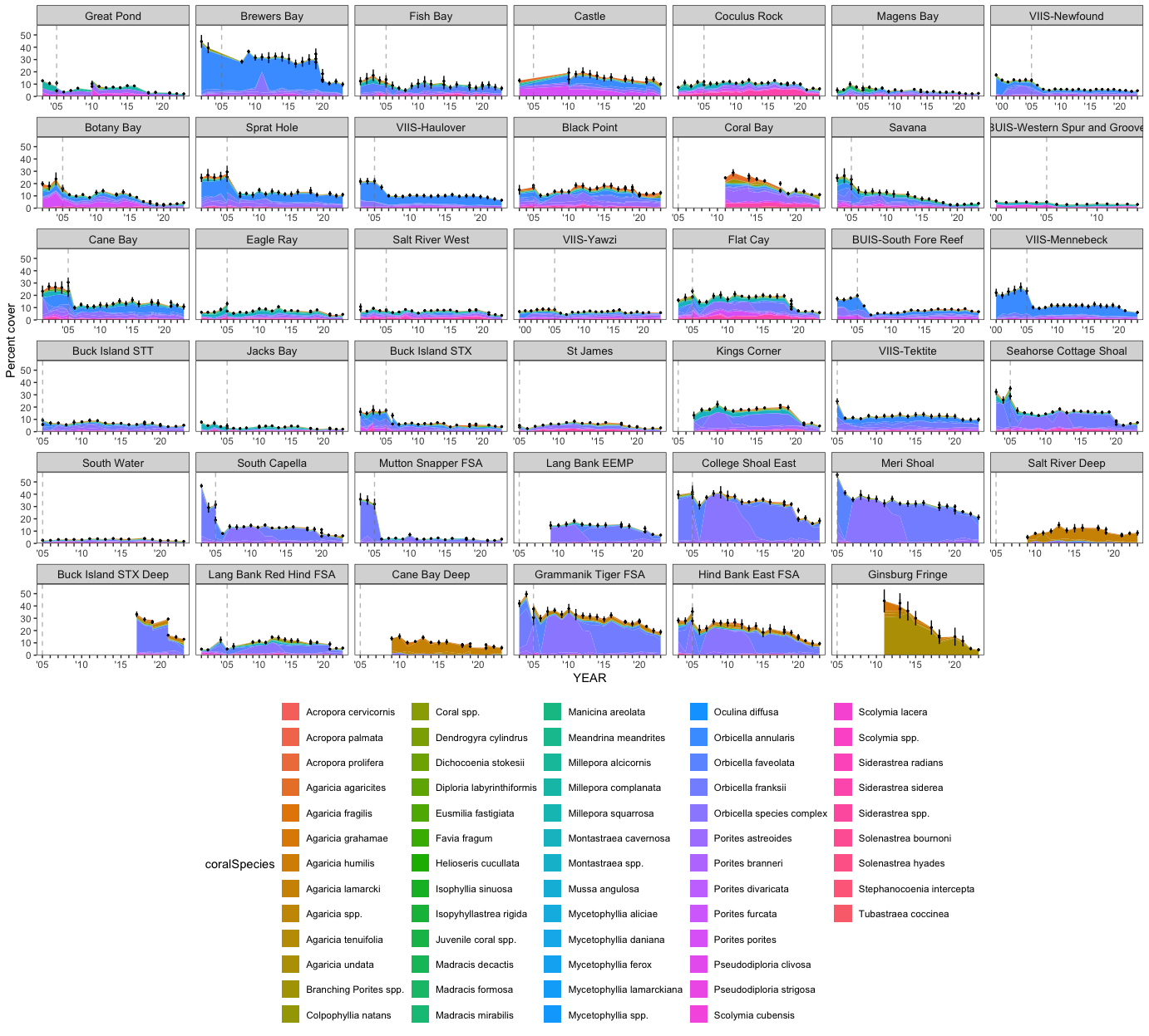
Total coral cover declined at most sites after the 2005 bleaching event, and a handful of species account for most of the remaining cover. The proportional view below (Figure 2) isolates the ten highest-cover species so the dominant species stand out.
We rank species by overall mean cover and keep the ten highest for the proportional plot.
# Calculate the overall mean coverage for each coralSpecies
top_species <- groupedBenthicDatCovSum |>
  group_by(coralSpecies) |>
  summarise(overall_meancov = mean(meancov, na.rm = TRUE)) |>
  arrange(-overall_meancov) |>
  head(10) |>
  pull(coralSpecies)

# Filter the original dataframe to only include the top 10 species
groupedBenthicDatCovSumTop <- groupedBenthicDatCovSum |>
  filter(coralSpecies %in% top_species)
groupedBenthicDatCovSumTop now holds only the records for the ten coral species with the highest overall mean cover. The ten species retained are Agaricia agaricites, Agaricia lamarcki, Montastraea cavernosa, Orbicella annularis, Orbicella faveolata, Orbicella franksii, Orbicella species complex, Porites astreoides, Porites porites, Siderastrea siderea.
create_proportional_stacked_area_plot() builds the site-faceted proportional plot: within each site panel it rescales the ten species to fill the panel height, so the panels show relative make-up rather than absolute cover.
create_proportional_stacked_area_plot <-
  function(data_stacked,
           x_var = "year",
           y_var = "meancov",
           fill_var = "coralSpecies",
           facet_var = "site",
           min_year = NULL,
           max_year = NULL,
           highlight_year = NULL,
           max_facets_per_page = 35) {
    # Determine x-axis limits if not provided
    if (is.null(min_year))
      min_year <- floor(min(data_stacked[[x_var]]))
    if (is.null(max_year))
      max_year <- ceiling(max(data_stacked[[x_var]]))

    # Calculate optimal number of rows and columns
    n_facets <- length(unique(data_stacked[[facet_var]]))
    n_facets <- min(n_facets, max_facets_per_page)  # Limit to max_facets_per_page
    n_col <- ceiling(sqrt(n_facets))
    n_row <- ceiling(n_facets / n_col)

    # Create base plot
    p <- ggplot(data_stacked, aes(x = .data[[x_var]], y = .data[[y_var]], fill = .data[[fill_var]])) +
      geom_area(position = 'fill') +
      facet_wrap(vars(.data[[facet_var]]), nrow = n_row, ncol = n_col, scales = "free_x") +
      labs(y = "Proportion", x = toupper(x_var)) +
      scale_y_continuous(expand = c(0, 0), labels = scales::percent) +
      scale_x_continuous(
        expand = expansion(mult = 0.04),
        breaks = seq(min_year, max_year, by = 1),
        labels = function(x)
          ifelse(x %% 5 == 0, paste0("'", substr(x, 3, 4)), "")
      ) +
      theme_bw() +
      theme(
        strip.text = element_text(size = 10),
        legend.position = "bottom",
        panel.grid = element_blank()
      )

    # Add highlight line if specified
    if (!is.null(highlight_year)) {
      p <- p + geom_vline(
        xintercept = highlight_year,
        color = "gray50",
        alpha = 0.5,
        linetype = "dashed"
      )
    }

    return(p)
  }
Figure 2 shows the proportional make-up of the ten highest-cover species at each site. Reading the panels shallow to deep shows how the dominant species shift with depth and over time.
This page writes the coral-species cover product s2pt5_benthicCoverCoralSpecies (one row per site, year, and species) plus its metadata. The download links below are generated from the same object the page computes. The metadata file carries the UAGA correction note so provenance travels with the data.
Derived data: s2pt5_benthicCoverCoralSpecies_41sites_1999_2023.csv (37.4 MB)
Metadata: s2pt5_benthicCoverCoralSpecies_41sites_1999_2023.txt
version 1.0.0 • in-review • data ≤ 2023