3.5 Coral biodiversity

Last updated

July 6, 2026

3.5 Coral biodiversity

On this page

This page turns the site-level coral cover series into coral biodiversity metrics and tracks them through time. We compute four diversity indices per program, site, replicate, and year: Species Richness (S), the Shannon Diversity Index (H’), Pielou’s Evenness Index (J’), and the Inverse Simpson Diversity Index (1/D), and we pair each metric with absolute coral cover at the same site and year. The page reads one benthic-cover output (the coral-species cover file) and writes one downstream product: a per-site, per-year table of the four diversity indices alongside absolute coral cover. That table is offered in the Downloads section below and feeds the resilience-values section. The figures show how diversity and cover move together across the monitoring record, through diversity ridgeline distributions (Figure 1 through Figure 4) and cover-versus-diversity relationships (Figure 13 and Figure 17).

Data sources

This page uses coral cover by species, derived from the TCRMP, VINPS, and CSUN monitoring programs and read from the benthic-cover section output s2pt5_benthicCoverCoralSpecies. The validation note below reports the exact site count, year range, programs, and species count for the cut this render used, and all records stay within the ≤ 2023 embargo window. This page’s own derived product, the per-site coral biodiversity table, is available in the Downloads section below.

WarningSampling structure differs by program

TCRMP and VINPS both survey along replicate transects, so replicate-level variation supports the standard error shown in the summarized figures. The two programs use distinct site sets and start years, so read each program’s series on its own footing rather than as one pooled trend.

Import data

We read the coral-species cover file and its metadata sidecar. The read path is set once here and reused by the download step at the bottom.

Show code
# file_coralcover <- "s2pt3_benthicCoverMajorBenthicCategories_35sites_2003_2022"
# Repointed (2026-07-04) from the now-absent s2pt5_...40sites_2001_2024 cut to the current
# benthic-cover output. The analysis now runs on 41 sites, 1999-2024. Numbers reflect this cut.
file_coralcover <- latest_output("s2pt5_benthicCoverCoralSpecies")

data_coralcover <- read.csv(paste("../../outputs/",file_coralcover,".csv",sep=""))
metadata_coralcover <- readLines(paste("../../outputs/",file_coralcover,".txt",sep=""))

Validation note. The loaded cover file holds 450,668 records across 41 sites and the years 1999 through 2023, from the TCRMP and VINPS programs, covering 61 coral species.

Derive metrics from coral cover

Absolute coral cover

What happens here: we sum species-level percent cover within each program, year, site, period, replicate, and date to get total absolute coral cover per transect survey.

Show code
# 1: Group the data by 'program', 'site', 'replicate', 'year', and 'date'
# 2: Calculate the sum of 'perccover' for each group
# 3: Create a new column 'coralcover_date' and set it equal to the 'date' column
# 4: Remove the 'date' column from the dataset
# 5: Ungroup the dataset, removing the grouping structure

mod_coralcover <- data_coralcover |> 
  group_by(program, year, site, period, replicate, date) |>
  summarise(coralcover = sum(perccover)) |>
  mutate(coralcover_date = date) |>
  select(-date) |>
  ungroup()

Inverse Simpson diversity

We calculate the Inverse Simpson Diversity Index for each combination of year, site, and replicate. This index summarizes the diversity of coral taxa observed during each survey, with higher values indicating greater diversity.

the Simpson Diversity Index (\(D\)):

\[D = \sum_{i=1}^{S} p_i^2\]

where:

  • \(p_i\) would be the proportion of each coralGenera in each year, site, and replicate, which can be calculated as the perccover of that coralGenera divided by the total perccover for that group.

  • \(S\) would be the number of unique coralGenera in that group.

This index calculates the probability that two randomly selected individuals (here, points) from the dataset will belong to the same species. A higher value of \(D\) implies lower diversity, as it indicates a higher probability of two individuals being of the same species.

And the inverse Simpson Diversity Index is:

\[D_{\text{inv}} = \frac{1}{D}\]

This value will increase as \(D\) decreases, meaning that higher diversity (more equal distribution among species) will result in a higher \(D_{\text{inv}}\). Conversely, lower diversity (one or few species dominating) will result in a lower \(D_{\text{inv}}\).

Show code
inverse_simpson_df <- data_coralcover |>
  group_by(program, year, site, replicate, coralSpecies) |>
  summarise(abundance = sum(perccover), .groups = 'drop') |>
  group_by(year, site, replicate) |>
  mutate(total_abundance = sum(abundance)) |>
  filter(total_abundance > 0) |>
  mutate(proportion = abundance / total_abundance) |>
  summarise(D = sum(proportion^2), .groups = 'drop') |>
  mutate(inverse_simpson = 1 / D)

Other useful metrics

We add three more indices:

  1. Species Richness (S): the total number of different species present in a community.
  2. Shannon Diversity Index (H’): accounts for both abundance and evenness of the species present.
  3. Pielou’s Evenness Index (J’): measures how evenly individuals are distributed among the species.

We calculate these metrics from the data_coralcover dataframe with the tidyverse package.

First, we calculate the abundance (percent cover) of each coral species per year, site, and replicate.

Show code
diversity_df <- data_coralcover |>
  group_by(program, year, site, period, replicate, coralSpecies) |>
  summarise(abundance = sum(perccover), .groups = 'drop')

We compute the total abundance per group and the proportion of each species.

Show code
diversity_df <- diversity_df |>
  group_by(program, year, site, period, replicate) |>
  mutate(
    total_abundance = sum(abundance),
    proportion = abundance / total_abundance
  ) |>
  filter(total_abundance > 0)

Species Richness (S)

Count the number of unique species per group.

Shannon Diversity Index (H’)

Use the formula:

\[ H' = -\sum_{i=1}^{S} p_i \ln p_i \]

Pielou’s Evenness Index (J’)

Calculated as:

\[ J' = \frac{H'}{\ln S} \]

Show code
diversity_metrics_df <- diversity_df |>
  mutate(
    p_ln_p = ifelse(proportion > 0, proportion * log(proportion), 0)
  ) |>
  group_by(program, year, site, period, replicate) |>
  filter(abundance>0) |>
  summarise(
    S = n_distinct(coralSpecies),               # Species Richness
    H = -sum(p_ln_p, na.rm = TRUE),             # Shannon Diversity Index
    .groups = 'drop'
  ) |>
  mutate(
    J = ifelse(S > 1, H / log(S), NA)           # Pielou's Evenness Index
  )

We set \(p_i \ln p_i = 0\) when \(p_i = 0\) to avoid NaN values.

If S is 1, log(S) is 0, so J is undefined (NA).

Combine with Inverse Simpson Index

We merge the Inverse Simpson Index into the richness, Shannon, and evenness table.

Show code
diversity_metrics_df <- diversity_metrics_df |>
  left_join(inverse_simpson_df, by = c("year", "site","replicate"))

Validation note. The combined metrics table holds 7,064 rows and 10 columns. Each row is one program-site-period-replicate-year survey carrying its Species Richness (S), Shannon Diversity (H), Pielou’s Evenness (J), Simpson’s Index (D), and Inverse Simpson (inverse_simpson).

What the metrics mean

  • Species Richness (S): The number of different species present.
  • Shannon Diversity Index (H’): Reflects both species abundance and evenness; higher values indicate greater diversity.
  • Pielou’s Evenness Index (J’): Values range from 0 (uneven distribution) to 1 (complete evenness).
  • Simpson’s Index (D): Measures the probability that two individuals randomly selected will belong to the same species; lower values mean higher diversity.
  • Inverse Simpson’s Index (1/D): Higher values indicate greater diversity, emphasizing dominant species.

Two further metrics are available for future use. Margalef’s Richness Index accounts for both the number of species and the number of individuals:

\[ D_M = \frac{S - 1}{\ln N} \]

where \(S\) is species richness and \(N\) is total abundance. Fisher’s Alpha models species abundance distributions.

Join metrics to coral cover

What happens here: we join the four diversity indices back onto the absolute cover table, so every transect survey carries both its total cover and its diversity metrics.

Show code
mod_coralcover <- mod_coralcover |>
  left_join(
    diversity_metrics_df,
    by = c("program", "site", "year", "period","replicate")
  )

Plots

Ridgeline distributions of diversity over time per site

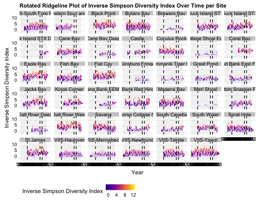
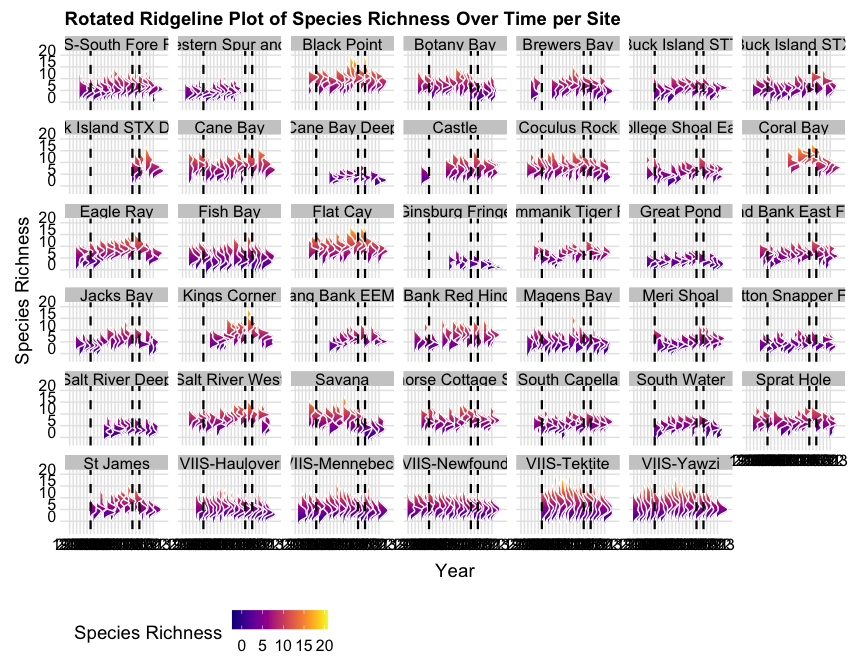
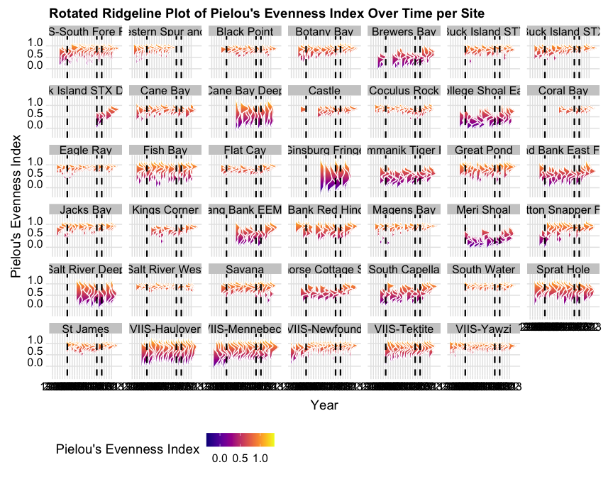
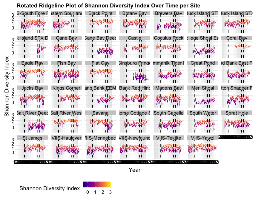
The ridgeline plots below show, for each site, how the distribution of a diversity metric shifts across survey years. Each row is one year, and the ridge shows the spread of replicate-level values for that year. Dashed reference lines mark the 2005 bleaching event, the 2017 hurricanes, and 2019. With 41 sites faceted, each panel is small; the interactive site picker proposed in the report is the better way to read any single site closely.

Show code
plot_diversity_ridgeline <- function(diversity_data,
                                     metric = "H",
                                     metric_label = "Shannon Diversity Index") {
  # Ensure 'year' is numeric for proper scaling
  diversity_data$year <- as.numeric(as.character(diversity_data$year))
  
  # Create the rotated ridgeline plot
  ggplot(diversity_data,
         aes_string(
           x = metric,
           y = "year",
           group = "year",
           fill = "..x.."
         )) +
    geom_density_ridges_gradient(scale = 3,
                                 rel_min_height = 0.01,
                                 color = "white") +
    coord_flip() +
    facet_wrap( ~ site) +
    scale_y_continuous(breaks = unique(diversity_data$year)) +
    scale_fill_viridis(name = metric_label, option = "C") +
    labs(
      title = paste("Rotated Ridgeline Plot of", metric_label, "Over Time per Site"),
      x = metric_label,
      y = "Year"
    ) +
    theme_ridges(center_axis_labels = TRUE) +
    theme(legend.position = "bottom") +
    geom_hline(
      yintercept = c(2005, 2017, 2019),
      color = "black",
      linetype = "dashed",
      size = 0.8
    )
}

The Shannon distribution per site over time is shown in Figure 1.

Show code
plot_diversity_ridgeline(mod_coralcover, metric = "H", metric_label = "Shannon Diversity Index")
Sec 3.5 Figure 1: Distribution of the Shannon Diversity Index (H’) by year at each site. Each ridge is one survey year; dashed lines mark 2005, 2017, and 2019.

The Inverse Simpson distribution per site over time is shown in Figure 2.

Show code
# Inverse Simpson Diversity Index
plot_diversity_ridgeline(mod_coralcover, metric = "inverse_simpson", metric_label = "Inverse Simpson Diversity Index")
Sec 3.5 Figure 2: Distribution of the Inverse Simpson Diversity Index (1/D) by year at each site. Higher values indicate greater diversity.

The Species Richness distribution per site over time is shown in Figure 3.

Show code
# Species Richness
plot_diversity_ridgeline(mod_coralcover, metric = "S", metric_label = "Species Richness")
Sec 3.5 Figure 3: Distribution of Species Richness (S), the count of coral species per replicate, by year at each site.

Pielou’s Evenness distribution per site over time is shown in Figure 4.

Show code
# Pielou's Evenness Index
plot_diversity_ridgeline(mod_coralcover, metric = "J", metric_label = "Pielou's Evenness Index")
Sec 3.5 Figure 4: Distribution of Pielou’s Evenness Index (J’) by year at each site. Values near 1 indicate even distribution among species.

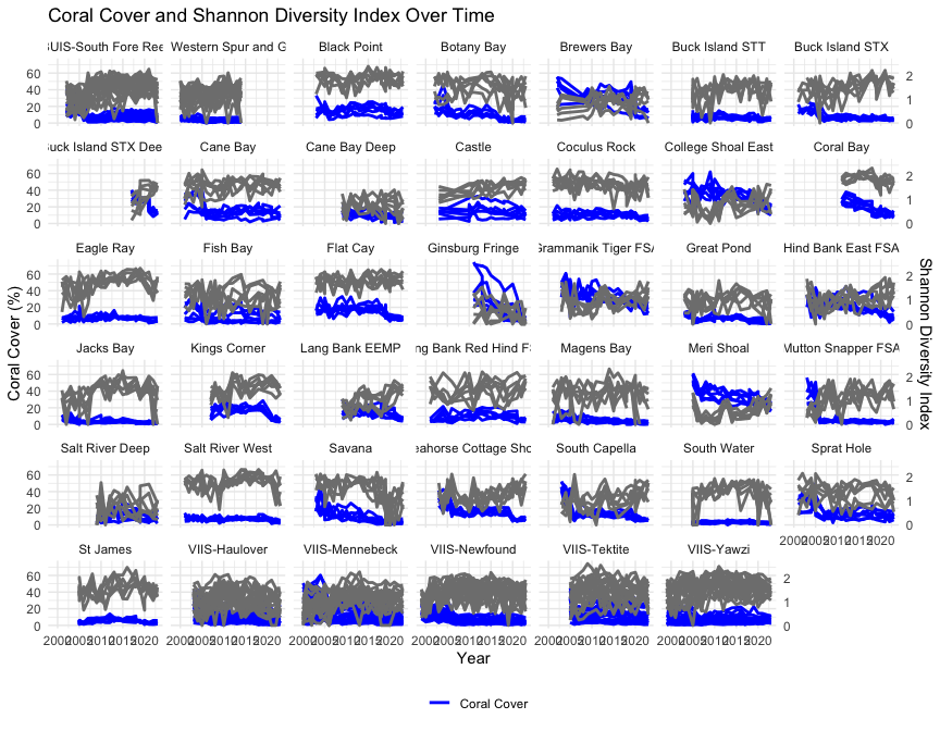
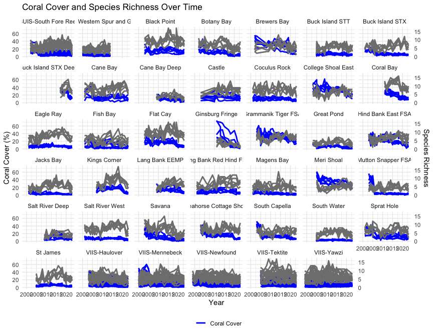
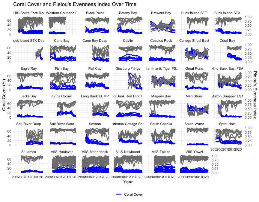
Raw coral cover and diversity over time at each transect

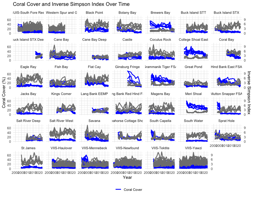
The next set of figures overlays absolute coral cover and one diversity metric on a shared time axis for each site, so periods of cover change can be read alongside diversity change. The two series use a secondary axis because they are on different scales.

Show code
plot_cover_and_metric <- function(data,
                                  metric = "inverse_simpson",
                                  metric_label = "Inverse Simpson Index",
                                  cover_column = "coralcover",
                                  group_var = "replicate",
                                  facet_var = "site") {

  # Calculate scale factor to align the two variables
  max_cover <- max(data[[cover_column]], na.rm = TRUE)
  max_metric <- max(data[[metric]], na.rm = TRUE)
  scale_factor <- max_cover / max_metric
  
  # Generate the plot
  ggplot(data, aes(x = year)) +
    geom_line(aes_string(
      y = cover_column,
      color = shQuote("Coral Cover"),
      group = group_var
    ),
    size = 1) +
    geom_line(aes_string(
      y = paste0(metric, " * scale_factor"),
      color = shQuote(metric_label),
      group = group_var
    ),
    size = 1) +
    scale_y_continuous(name = "Coral Cover (%)",
                       sec.axis = sec_axis( ~ . / scale_factor, name = metric_label)) +
    scale_color_manual(name = "",
                       values = c("Coral Cover" = "blue", metric_label = "red")) +
    facet_wrap(as.formula(paste("~", facet_var))) +
    labs(title = paste("Coral Cover and", metric_label, "Over Time"),
         x = "Year") +
    theme_minimal() +
    theme(legend.position = "bottom")
}

Raw coral cover against the Inverse Simpson Index per site is shown in Figure 5.

Show code
plot_cover_and_metric(mod_coralcover, metric = "inverse_simpson", metric_label = "Inverse Simpson Index")
Sec 3.5 Figure 5: Raw coral cover (blue) and the Inverse Simpson Index (red) over time at each site. Left axis: coral cover (%); right axis: index.

Raw coral cover against the Shannon Diversity Index per site is shown in Figure 6.

Show code
plot_cover_and_metric(mod_coralcover, metric = "H", metric_label = "Shannon Diversity Index")
Sec 3.5 Figure 6: Raw coral cover (blue) and the Shannon Diversity Index (red) over time at each site.

Raw coral cover against Species Richness per site is shown in Figure 7.

Show code
plot_cover_and_metric(mod_coralcover, metric = "S", metric_label = "Species Richness")
Sec 3.5 Figure 7: Raw coral cover (blue) and Species Richness (red) over time at each site.

Raw coral cover against Pielou’s Evenness Index per site is shown in Figure 8.

Show code
plot_cover_and_metric(mod_coralcover, metric = "J", metric_label = "Pielou's Evenness Index")
Sec 3.5 Figure 8: Raw coral cover (blue) and Pielou’s Evenness Index (red) over time at each site.

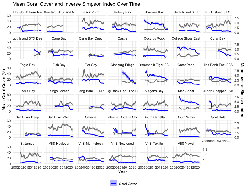
Summarized coral cover and diversity over time at each site

The summarized figures average the replicate-level values to one mean per site and year, with a standard-error ribbon. Because both TCRMP and VINPS survey replicate transects, the standard error is supported here.

Show code
calculate_summary_stats <- function(data,
                                    metric = "inverse_simpson",
                                    group_vars = c("site", "year")) {
  summary_data <- data %>%
    group_by(across(all_of(group_vars))) %>%
    summarise(
      mean_coralcover = mean(coralcover, na.rm = TRUE),
      se_coralcover = sd(coralcover, na.rm = TRUE) / sqrt(n()),
      mean_metric = mean(get(metric), na.rm = TRUE),
      se_metric = sd(get(metric), na.rm = TRUE) / sqrt(n()),
      .groups = 'drop'
    )
  
  return(summary_data)
}

plot_mean_and_se <- function(summary_data,
                             metric_label = "Inverse Simpson Index",
                             facet_var = "site",
                             smooth = FALSE) {
  # Calculate scale factor to align the two variables
  max_coralcover <- max(summary_data$mean_coralcover, na.rm = TRUE)
  max_metric <- max(summary_data$mean_metric, na.rm = TRUE)
  scale_factor <- max_coralcover / max_metric
  
  p <- ggplot(summary_data, aes(x = year))
  
  if (smooth) {
    # Smoothed lines with confidence intervals
    p <- p +
      geom_smooth(
        aes(
          y = mean_coralcover,
          color = "Coral Cover",
          fill = "Coral Cover"
        ),
        method = "loess",
        span = 0.5,
        se = TRUE,
        alpha = 0.2
      ) +
      geom_smooth(
        aes(
          y = mean_metric * scale_factor,
          color = metric_label,
          fill = metric_label
        ),
        method = "loess",
        span = 0.5,
        se = TRUE,
        alpha = 0.2
      )
  } else {
    # Mean lines with error ribbons
    p <- p +
      geom_line(aes(y = mean_coralcover, color = "Coral Cover"), size = 1) +
      geom_ribbon(
        aes(
          ymin = mean_coralcover - se_coralcover,
          ymax = mean_coralcover + se_coralcover,
          fill = "Coral Cover"
        ),
        alpha = 0.3
      ) +
      geom_line(aes(y = mean_metric * scale_factor, color = metric_label),
                size = 1) +
      geom_ribbon(aes(
        ymin = (mean_metric - se_metric) * scale_factor,
        ymax = (mean_metric + se_metric) * scale_factor,
        fill = metric_label
      ),
      alpha = 0.3)
  }
  
  p <- p +
    scale_y_continuous(name = "Mean Coral Cover (%)",
                       sec.axis = sec_axis( ~ . / scale_factor, name = paste("Mean", metric_label))) +
    scale_color_manual(name = "",
                       values = c("Coral Cover" = "blue", metric_label = "red")) +
    scale_fill_manual(name = "",
                      values = c("Coral Cover" = "blue", metric_label = "red")) +
    facet_wrap(as.formula(paste("~", facet_var))) +
    labs(title = paste("Mean Coral Cover and", metric_label, "Over Time"),
         x = "Year") +
    theme_minimal() +
    theme(legend.position = "bottom")
  
  return(p)
}
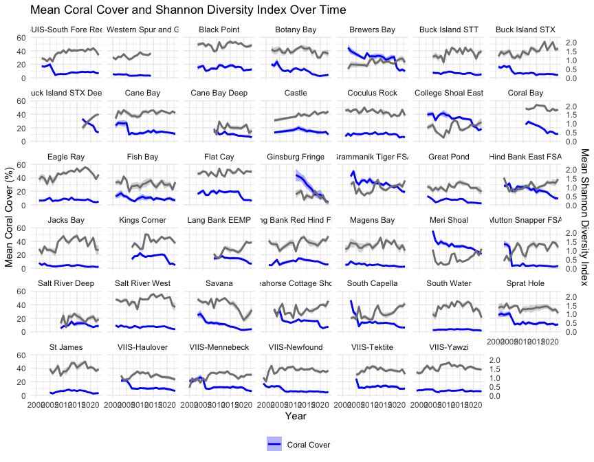
Mean coral cover and the Inverse Simpson Index, with standard-error ribbons, are shown in Figure 9.

Show code
plot_mean_and_se(
  calculate_summary_stats(mod_coralcover, metric = "inverse_simpson"),
  metric_label = "Inverse Simpson Index",
  smooth = FALSE
)
Sec 3.5 Figure 9: Mean coral cover (blue) and mean Inverse Simpson Index (red) over time at each site, with standard-error ribbons.

Mean coral cover and the Shannon Diversity Index are shown in Figure 10.

Show code
plot_mean_and_se(
  calculate_summary_stats(mod_coralcover, metric = "H"),
  metric_label = "Shannon Diversity Index",
  smooth = FALSE
)
Sec 3.5 Figure 10: Mean coral cover (blue) and mean Shannon Diversity Index (red) over time at each site, with standard-error ribbons.

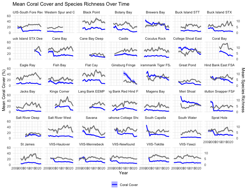
Mean coral cover and Species Richness are shown in Figure 11.

Show code
plot_mean_and_se(
  calculate_summary_stats(mod_coralcover, metric = "S"),
  metric_label = "Species Richness",
  smooth = FALSE
)
Sec 3.5 Figure 11: Mean coral cover (blue) and mean Species Richness (red) over time at each site, with standard-error ribbons.

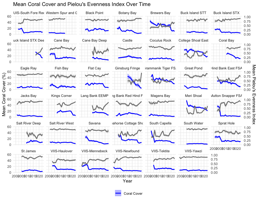
Mean coral cover and Pielou’s Evenness Index are shown in Figure 12.

Show code
plot_mean_and_se(
  calculate_summary_stats(mod_coralcover, metric = "J"),
  metric_label = "Pielou's Evenness Index",
  smooth = FALSE
)
Sec 3.5 Figure 12: Mean coral cover (blue) and mean Pielou’s Evenness Index (red) over time at each site, with standard-error ribbons.

Relationship between coral cover and diversity at each site

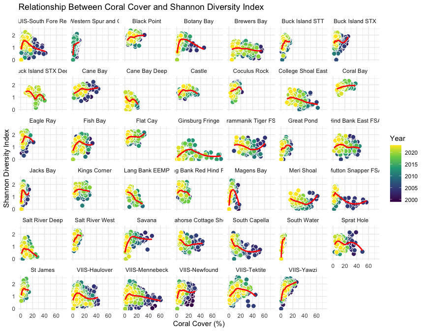
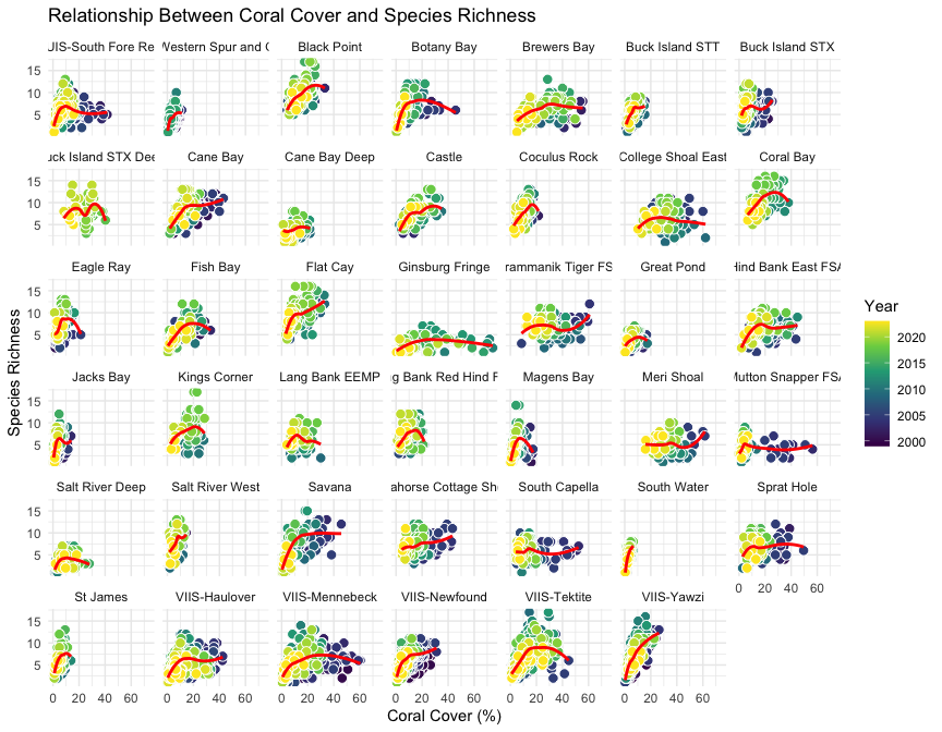
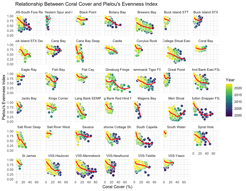
These scatter panels plot each survey’s diversity metric against its coral cover, one panel per site, with a loess trend. Point color encodes year, so the reader can see whether the cover-diversity relationship has drifted over the record.

Show code
plot_relationship <- function(data,
                              x_var = "coralcover",
                              y_var = "inverse_simpson",
                              x_label = "Coral Cover (%)",
                              y_label = "Inverse Simpson Index",
                              title = "Relationship Between Coral Cover and Inverse Simpson Index",
                              facet_var = "site",
                              smooth_method = "loess",
                              point_alpha = 1) {
  ggplot(data, aes_string(x = x_var, y = y_var)) +
    geom_point(
      aes(fill = year),
      alpha = point_alpha,
      pch = 21,
      size = 3,
      color = "white"
    ) +
    scale_fill_viridis_c(name = "Year") +
    geom_smooth(method = smooth_method,
                se = FALSE,
                color = "red") +
    facet_wrap(as.formula(paste("~", facet_var))) +
    labs(title = title, x = x_label, y = y_label) +
    theme_minimal()
}

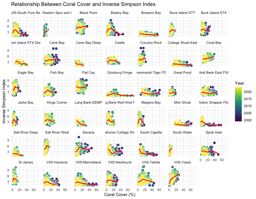
The per-site relationship between coral cover and the Inverse Simpson Index is shown in Figure 13.

Show code
# inverse simpson
plot_relationship(mod_coralcover)
Sec 3.5 Figure 13: Inverse Simpson Index against coral cover at each site, colored by year, with a loess trend.

The per-site relationship with the Shannon Diversity Index is shown in Figure 14.

Show code
# shannon
plot_relationship(mod_coralcover,
                  y_var = "H",
                  y_label = "Shannon Diversity Index",
                  title = "Relationship Between Coral Cover and Shannon Diversity Index")
Sec 3.5 Figure 14: Shannon Diversity Index against coral cover at each site, colored by year, with a loess trend.

The per-site relationship with Species Richness is shown in Figure 15.

Show code
# species richness
plot_relationship(mod_coralcover,
                  y_var = "S",
                  y_label = "Species Richness",
                  title = "Relationship Between Coral Cover and Species Richness")
Sec 3.5 Figure 15: Species Richness against coral cover at each site, colored by year, with a loess trend.

The per-site relationship with Pielou’s Evenness Index is shown in Figure 16.

Show code
#pielou's evenness
plot_relationship(mod_coralcover,
                  y_var = "J",
                  y_label = "Pielou's Evenness Index",
                  title = "Relationship Between Coral Cover and Pielou's Evenness Index")
Sec 3.5 Figure 16: Pielou’s Evenness Index against coral cover at each site, colored by year, with a loess trend.

Relationship between coral cover and diversity across all sites

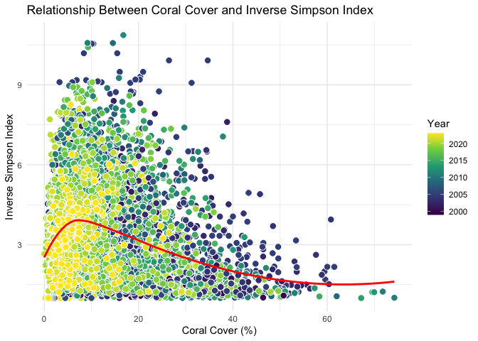
Pooling all sites into one panel shows the overall shape of the cover-diversity relationship across the whole record.

Show code
plot_relationship_all <- function(data,
                                  x_var = "coralcover",
                                  y_var = "inverse_simpson",
                                  x_label = "Coral Cover (%)",
                                  y_label = "Inverse Simpson Index",
                                  title = "Relationship Between Coral Cover and Inverse Simpson Index",
                                  smooth_method = "loess",
                                  point_alpha = 1) {
  ggplot(data, aes_string(x = x_var, y = y_var)) +
    geom_point(
      aes(fill = year),
      alpha = point_alpha,
      pch = 21,
      size = 3,
      color = "white"
    ) +
    scale_fill_viridis_c(name = "Year") +
    geom_smooth(method = smooth_method,
                se = FALSE,
                color = "red") +
    # facet_wrap(as.formula(paste("~", facet_var))) +
    labs(title = title, x = x_label, y = y_label) +
    theme_minimal()
}

The pooled relationship between coral cover and the Inverse Simpson Index is shown in Figure 17.

Show code
# inverse simpson
plot_relationship_all(mod_coralcover)
Sec 3.5 Figure 17: Inverse Simpson Index against coral cover across all sites, colored by year, with a loess trend.
TipKey result

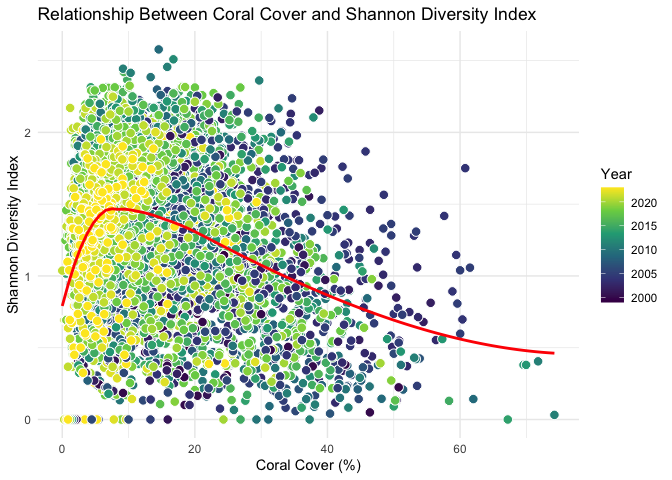
Across all sites and years, diversity and absolute coral cover are not tightly coupled: high-cover surveys span a wide range of diversity, and the loess trend is shallow. Coral cover on its own is a weak predictor of how many coral species a site holds.

The pooled relationship with the Shannon Diversity Index is shown in Figure 18.

Show code
# shannon diversity
plot_relationship_all(mod_coralcover,
                  y_var = "H",
                  y_label = "Shannon Diversity Index",
                  title = "Relationship Between Coral Cover and Shannon Diversity Index")
Sec 3.5 Figure 18: Shannon Diversity Index against coral cover across all sites, colored by year, with a loess trend.

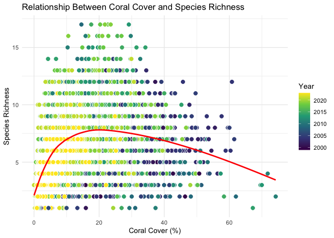
The pooled relationship with Species Richness is shown in Figure 19.

Show code
# species richness
plot_relationship_all(mod_coralcover,
                  y_var = "S",
                  y_label = "Species Richness",
                  title = "Relationship Between Coral Cover and Species Richness")
Sec 3.5 Figure 19: Species Richness against coral cover across all sites, colored by year, with a loess trend.

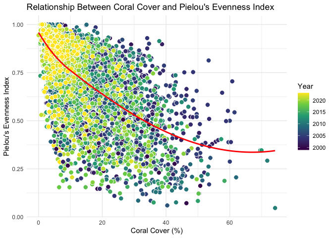
The pooled relationship with Pielou’s Evenness Index is shown in Figure 20.

Show code
# pielou's evenness
plot_relationship_all(mod_coralcover,
                  y_var = "J",
                  y_label = "Pielou's Evenness Index",
                  title = "Relationship Between Coral Cover and Pielou's Evenness Index")
Sec 3.5 Figure 20: Pielou’s Evenness Index against coral cover across all sites, colored by year, with a loess trend.

Other plots (not evaluated here)

The footnote below sketches additional visualizations (a heatmap, a 3D scatter, an animation, a radial bar chart, and a mirrored ridgeline) that are kept as code but not rendered.1

Downloads

The links below offer this page’s derived coral biodiversity table, its metadata, and this page’s .qmd source.


version 1.0.0 • in-review • data ≤ 2023-12-31

Footnotes

  1. ```{r, eval = FALSE} ggplot(mod_coralcover, aes(x = factor(year), y = factor(replicate))) + geom_tile(aes(fill = coralcover)) + geom_text(aes(label = round(inverse_simpson, 2)), color = “white”) + facet_wrap(~ site) + scale_fill_viridis_c(name = “Coral Cover (%)”) + labs(title = “Heatmap of Coral Cover with Inverse Simpson Index”, x = “Year”, y = “Replicate”) + theme_minimal() library(plotly)

    plot_ly(mod_coralcover, x = ~year, y = ~coralcover, z = ~inverse_simpson, type = ‘scatter3d’, mode = ‘markers’, color = ~site, marker = list(size = 3)) %>% layout(title = “3D Scatter Plot of Coral Cover and Inverse Simpson Index Over Time”, scene = list(xaxis = list(title = ‘Year’), yaxis = list(title = ‘Coral Cover (%)’), zaxis = list(title = ‘Inverse Simpson Index’))) library(gganimate)

    ggplot(mod_coralcover, aes(x = coralcover, y = inverse_simpson, color = site)) + geom_point(size = 3) + transition_time(year) + labs(title = “Year: {frame_time}”, x = “Coral Cover (%)”, y = “Inverse Simpson Index”) + theme_minimal()

    ggplot(mod_coralcover, aes(x = factor(year), y = coralcover, fill = inverse_simpson)) + geom_bar(stat = “identity”, width = 1) + coord_polar() + facet_wrap(~ site) + scale_fill_viridis_c(name = “Inverse Simpson Index”) + labs(title = “Radial Bar Chart of Coral Cover and Diversity”, x = ““, y =”Coral Cover (%)“) + theme_minimal() mod_coralcover\(year <- as.numeric(as.character(mod_coralcover\)year)) Create the mirrored ridgeline plot ggplot() + # Coral Cover Ridgelines (Upwards) geom_density_ridges( data = mod_coralcover, aes( x = coralcover, y = year, group = year, fill =”Coral Cover” ), scale = 1, rel_min_height = 0.01, color = “white”, alpha = 0.7 ) + # Inverse Simpson Index Ridgelines (Downwards, mirrored) geom_density_ridges( data = mod_coralcover, aes( x = -inverse_simpson, # Negate to mirror y = year, group = year, fill = “Inverse Simpson Index” ), scale = 1, rel_min_height = 0.01, color = “white”, alpha = 0.7 ) + # Vertical line at x = 0 to separate the mirrored ridgelines geom_vline(xintercept = 0, color = “black”, size = 0.5) + # Facet by site facet_wrap(~ site) + # Define manual fill colors for each variable scale_fill_manual( name = “Variable”, values = c(“Coral Cover” = “steelblue”, “Inverse Simpson Index” = “darkorange”) ) + # Adjust x-axis labels and breaks scale_x_continuous( name = “Value”, breaks = c( -max(mod_coralcover\(inverse_simpson, na.rm = TRUE), -mean(mod_coralcover\)inverse_simpson, na.rm = TRUE), 0, mean(mod_coralcover\(coralcover, na.rm = TRUE), max(mod_coralcover\)coralcover, na.rm = TRUE) ), labels = c( paste0(“High”, “190”), # Arrow pointing left “Inverse Simpson”, “0”, “Coral Cover”, paste0(“192”, ” High”) # Arrow pointing right ) ) + # Labels and theme adjustments labs( title = “Mirrored Ridgeline Plot of Coral Cover and Inverse Simpson Diversity Index Over Time”, y = “Year” ) + theme_ridges(center_axis_labels = TRUE) + theme( legend.position = “bottom”, axis.title.x = element_blank() ) ```↩︎