Show code
sitedat <-
  read.csv(
    "../../../RRSdata/00_RRS_dataCatalogStatus/00_RRS_siteMaster_allSites_data.csv"
)This page places whole-community benthic cover in a multivariate frame. We read five benthic-cover output families (coral, algae, sponge, zoanthid/gorgonians, and other), reduce each to a per-site, per-year mean percent cover of coral, algae, sponge, turf, and non-living substrate, then run a non-metric multidimensional scaling (NMDS) ordination on the community matrix and cluster the sites with k-means. The page produces one downloadable product, benthicOrganismCommunityCluster, holding the NMDS coordinates, k-means cluster assignment, and the per-site per-year cover values, along with the site-trajectory NMDS with cluster hulls (Figure 1) and the per-cluster cover-over-time panel. The community composition serves as a candidate response variable for later resilience analyses.
This page reads the benthic-cover section outputs (s2pt4 coral genera, s2pt7 algae taxa, s2pt8 sponge morphs, s2pt9 zoanthid/gorgonians, and s2pt10 other) joined to the RRS site master, and it scopes the community matrix to TCRMP and VINPS sites over the 2004 through 2017 recovery window (CSUN sites and Castle are dropped). The clustered product derived here is written to outputs/ and offered in the Downloads section below.
Under review. The five benthic-cover reads were repointed on 2026-07-04 from now-absent 35-site and 29-site 2003-2018 cuts to the current 49-site and 41-site cuts through 2023, matched by taxon name (the output section indices shifted). The downstream site set, NMDS ordination, clusters, and figures therefore reflect the new cuts and need Lauren’s scientific review before this page is treated as final.
We import the site master (sitedat) first.
sitedat <-
read.csv(
"../../../RRSdata/00_RRS_dataCatalogStatus/00_RRS_siteMaster_allSites_data.csv"
)We read the five benthic-cover output families, one per organism group.
# Repointed (2026-07-04) to the current benthic-cover outputs, matched by taxon (output indices
# shifted since the old cut). Now 49/41 sites through 2023 instead of the absent 35/29-site 2003-2018.
coral_df <-
  read_csv(paste0("../../outputs/", latest_output("s2pt4_benthicCoverCoralGenera"), ".csv"))
algae_df <-
  read_csv(paste0("../../outputs/", latest_output("s2pt7_benthicCoverAlgaeTaxa"), ".csv"))
sponge_df <-
  read_csv(paste0("../../outputs/", latest_output("s2pt8_benthicCoverSpongeMorphs"), ".csv"))
zoanthid_gorgonians_df <-
  read_csv(paste0("../../outputs/", latest_output("s2pt9_benthicCoverZoanthidGorgonians"), ".csv"))
other_df <-
  read_csv(paste0("../../outputs/", latest_output("s2pt10_benthicCoverOther"), ".csv"))
We define the species and category members that make up each functional group.
zoantharia_species <-
  c("Palythoa caribaeorum",
    "Zoanthids",
    "Zoanthus sociatus")

gorgonians_species <-
  c(
    "Briareum asbestinum",
    "Erythropodium caribaeorum",
    "Encrusting Gorgonian",
    "Sea fan",
    "Gorgonian",
    "Sea plume",
    "Sea rod",
    "Sea whip"
  )

non_living <-
  c("Boulder",
    "Pavement",
    "Rubble",
    "Sand")
We reduce each group to a per-site, per-year mean percent cover, averaging over transect replicates.
coral_cover <-
  coral_df |>
  group_by(site, year, replicate) |>
  summarise(perccover = sum(perccover)) |>
  group_by(site, year) |>
  summarise(coral = mean(perccover))

algae_cover <-
  algae_df |>
  group_by(site, year, replicate) |>
  summarise(perccover = sum(perccover)) |>
  group_by(site, year) |>
  summarise(algae = mean(perccover))

sponge_cover <-
  sponge_df |>
  group_by(site, year, replicate) |>
  summarise(perccover = sum(perccover)) |>
  group_by(site, year) |>
  summarise(sponge = mean(perccover))

zoantharia_cover <-
  zoanthid_gorgonians_df |>
  filter(zoanthidsGorgonians %in% zoantharia_species) |>
  group_by(site, year, replicate) |>
  summarise(perccover = sum(perccover)) |>
  group_by(site, year) |>
  summarise(zoantharian = mean(perccover))

gorgonians_cover <-
  zoanthid_gorgonians_df |>
  filter(zoanthidsGorgonians %in% gorgonians_species) |>
  group_by(site, year, replicate) |>
  summarise(perccover = sum(perccover)) |>
  group_by(site, year) |>
  summarise(gorgonian = mean(perccover))

turf_cover <-
  other_df |>
  filter(other == "Epilithic algae community") |>
  group_by(site, year, replicate) |>
  summarise(perccover = sum(perccover)) |>
  group_by(site, year) |>
  summarise(turf = mean(perccover))

non_living_cover <-
  other_df |>
  filter(other %in% non_living) |>
  group_by(site, year, replicate) |>
  summarise(perccover = sum(perccover)) |>
  group_by(site, year) |>
  summarise(nonliving = mean(perccover))
We join the group covers into one community table, fill missing cells with zero, then keep the TCRMP and VINPS sites over the recovery window.
# Start with the largest dataframe and left join the others one by one
cover <- coral_cover |>
  left_join(algae_cover, by = c("site", "year")) |>
  left_join(sponge_cover, by = c("site", "year")) |>
  # left_join(zoantharia_cover, by = c("site", "year")) |>
  # left_join(gorgonians_cover, by = c("site", "year")) |>
  left_join(turf_cover, by = c("site", "year")) |>
  left_join(non_living_cover, by = c("site", "year"))

# replace NA values with 0 if needed
cover <-
  cover |> replace_na(list(
    coral = 0,
    algae = 0,
    sponge = 0,
    # zoantharian = 0,
    # gorgonian = 0,
    turf = 0,
    nonliving = 0
  ))

# remove csun sites that only had algae and coral cover
# also only want recovery period
cover <- cover |>
  left_join(sitedat |> select(site, program), by = "site") |>
  filter(program != "CSUN") |>
  filter(year > 2003 & year < 2018) |>
  filter(site != "Castle")

rm(list = ls()[grep("_cover", ls())])
rm(list = ls()[grep("_df", ls())])We ordinate the site-by-year community records with non-metric multidimensional scaling (NMDS) on Bray-Curtis distances using metaMDS from the vegan package, then cluster the ordinated sites with k-means.
We prepare the data first: drop the non-numeric columns (site, year, and the trailing program column) and cast the community table to a numeric matrix, one row per site-year.
We run the NMDS in two dimensions with up to 40 random starts.
nmds_result <-
  metaMDS(data_matrix,
          distance = "bray",
          k = 2,
          trymax = 40,
          trace = FALSE)
The ordination reached a stress of 0.196 on 467 site-year records across 5 cover variables. Lower stress means the two-dimensional layout preserves the community distances more faithfully.
We assign the site-year points to five clusters with k-means.
We extract the NMDS coordinates and reorder sites shallow to deep for later plotting.
# Extract NMDS coordinates
nmds_coordinates <-
  as.data.frame(scores(nmds_result, display = "sites"))

#continuous grouping var
nmds_coordinates$site <- as.factor(cover$site)
nmds_coordinates$year <- as.factor(cover$year)
nmds_coordinates$cluster <- as.factor(cluster)

#join with depth for reordering
nmds_coordinates <- nmds_coordinates |>
  left_join(sitedat |> select(site, depth), by = "site")
nmds_coordinates <-
  nmds_coordinates[order(nmds_coordinates$depth),]
nmds_coordinates$site <-
  factor(nmds_coordinates$site, levels = unique(nmds_coordinates$site))

nmds_coordinates <- nmds_coordinates |>
arrange(site, year)We keep every year of a site in one cluster by clustering on site averages, so each site contributes one representative point. After the cluster of each site is set, we assign all of that site’s site-year points to the same cluster.
library(cluster)

# 1. Aggregate data by site
aggregated_data <- nmds_coordinates |>
  group_by(site) |>
  summarise(NMDS1_avg = mean(NMDS1), NMDS2_avg = mean(NMDS2))

# 2. Perform clustering on aggregated data
# Here, we're using k-means clustering as an example, with 3 clusters
set.seed(123)  # For reproducibility

clusters_result <-
  kmeans(aggregated_data[, c("NMDS1_avg", "NMDS2_avg")], centers = 4)

# 3. Assign clusters to original data
nmds_coordinates$cluster <-
  clusters_result$cluster[match(nmds_coordinates$site, aggregated_data$site)]
Each row of nmds_coordinates now carries a cluster column, and every year of a site shares that site’s cluster. We use this grouping in the figures below.
The NMDS site trajectories show how each site’s community moved through the recovery window, with a convex hull shading each k-means cluster (Figure 1). Sites that track together in the ordination share benthic community composition, and the hulls group those trajectories into clusters.
grouped_df <- nmds_coordinates |>
  distinct(site, cluster) |>
  mutate(clust_site = paste("clust", cluster, "-", gsub(" ", "_", site), sep =
                              ""))

nmds_coordinates <- nmds_coordinates |>
  left_join(grouped_df, by = c("site", "cluster"))

nmds_coordinates <- nmds_coordinates |>
  arrange(clust_site, year)

# Compute the convex hull for each cluster and preserve cluster IDs
hulls <- nmds_coordinates |>
  group_by(cluster) |>
  group_map(~ cbind(.x[chull(.x$NMDS1, .x$NMDS2), ], cluster = unique(.x$cluster)), .keep = TRUE) |>
  bind_rows()

hulls$cluster <- hulls[, ncol(hulls)]

# Create a ggplot
p1 <- ggplot(nmds_coordinates, aes(x = NMDS1, y = NMDS2)) +
  geom_polygon(
    data = hulls,
    aes(fill = as.factor(cluster), group = cluster),
    alpha = 0.4,
    show.legend = F
  ) +
  geom_path(aes(group = factor(site), color = factor(site)), linewidth = 0.5,) +
  geom_point(aes(color = factor(site), size = year), show.legend = F) +
  theme_minimal() +
  labs(color = "Cluster", fill = "Cluster") +
  xlab("NMDS Axis 1") +
  ylab("NMDS Axis 2") +
  theme_bw() +
  labs(color = "site",
       shape = "group",
       size = "year") +
  theme(legend.position = "bottom")

p1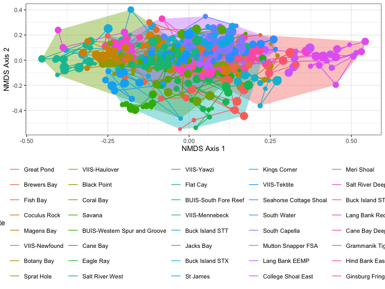
We build the year-to-year segments for an animated ordination trajectory.
# Ensure data is sorted by site and year
nmds_coordinates <- nmds_coordinates |> arrange(clust_site, year)

# Create a new dataframe for segments
segments <- nmds_coordinates |>
  group_by(site) |>
  # mutate(xend = lead(NMDS1), yend = lead(NMDS2))
  mutate(xend = lag(NMDS1), yend = lag(NMDS2))

# Remove rows where xend or yend is NA (i.e., the last year for each site)
segments <- segments |> filter(!is.na(xend) & !is.na(yend))
The animated NMDS steps through the years, tracing each cluster’s movement through community space (Figure 2).
library(gganimate)

p <- ggplot() +
  geom_point(data = nmds_coordinates,
             aes(
               x = NMDS1,
               y = NMDS2,
               color = factor(cluster)
             ),
             size = 4) +
  geom_segment(
    data = segments,
    aes(
      x = xend,
      y = yend,
      xend = NMDS1,
      yend = NMDS2,
      color = factor(cluster),
      group = year
    ),
    size = 1
  ) +
  transition_states(year) +
  shadow_trail(exclude_layer = 1) +
  xlab("NMDS Axis 1") +
  ylab("NMDS Axis 2") +
  theme_minimal() +
  labs(color = "depth",
       size = "relief") +
  enter_fade() +
  exit_fade() +
  theme(legend.position = "none") +
  ggtitle('{closest_state}')

p

# anim_save("biplot_animation.gif", p)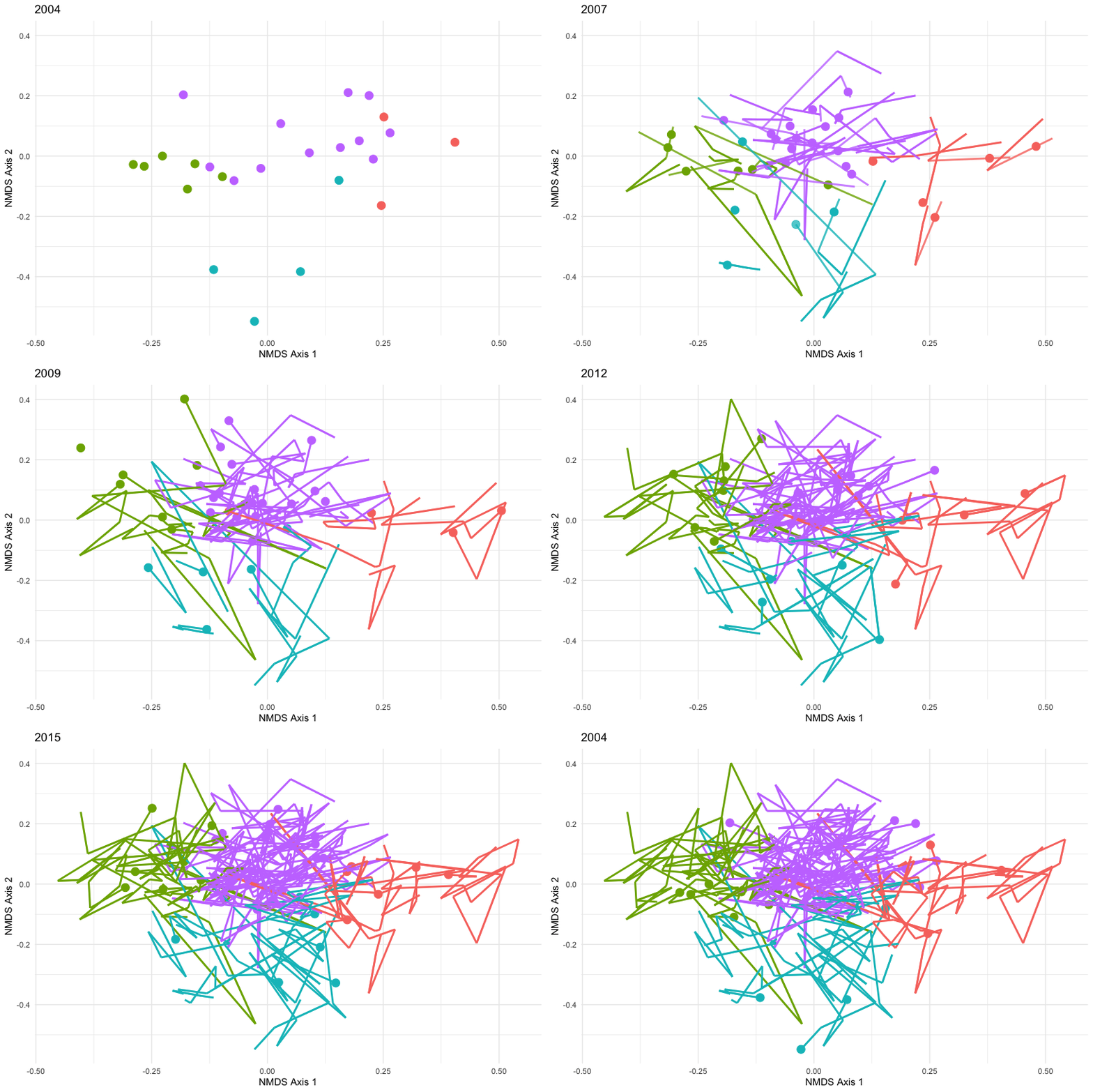
We join the cover values back to nmds_coordinates for export, then summarize each cluster’s coral, algae, sponge, and turf cover over time. The per-cluster panel pairs the ordination (left) with mean cover trajectories and standard-deviation ribbons for each cluster (the figure below), so the community differences that separate the clusters become legible as cover values.
cover$year <- factor(cover$year)

nmds_coordinates <- nmds_coordinates |>
  left_join(cover, by = c("site", "year"))


q <- nmds_coordinates |>
  group_by(cluster, year) |>
  summarise(
    meancoral = mean(coral),
    meanalgae = mean(algae),
    meansponge = mean(sponge),
    meanturf = mean(turf)
  ) |>
  ggplot(aes(x = year)) +
  geom_line(aes(y = meancoral, group = cluster), color = "goldenrod") +
  geom_line(aes(y = meanalgae, group = cluster), color = "green") +
  geom_line(aes(y = meansponge, group = cluster), color = "red") +
  geom_line(aes(y = meanturf, group = cluster), color = "brown") +
  facet_wrap( ~ cluster) +
  theme_bw() +
  ylab("percent cover")

# Calculate mean, sd, and ribbon limits for each variable
summary_data <- nmds_coordinates |>
  group_by(cluster, year) |>
  summarise(
    meancoral = mean(coral),
    sdcoral = sd(coral),
    meanalgae = mean(algae),
    sdalgae = sd(algae),
    meansponge = mean(sponge),
    sdsponge = sd(sponge),
    meanturf = mean(turf),
    sdturf = sd(turf),
    .groups = 'drop'
  )

# Plot with ribbons for each variable
q <- ggplot(summary_data, aes(x = year, group = cluster)) +
  geom_ribbon(
    aes(
      y = meancoral,
      ymin = meancoral - sdcoral,
      ymax = meancoral + sdcoral
    ),
    alpha = 0.2,
    fill = "goldenrod"
  ) +
  geom_line(aes(y = meancoral, group = cluster), color = "goldenrod") +

  geom_ribbon(aes(
    ymin = meanalgae - sdalgae,
    ymax = meanalgae + sdalgae,
    fill = "green"
  ),
  alpha = 0.2) +
  geom_line(aes(y = meanalgae, group = cluster), color = "green") +

  geom_ribbon(aes(
    ymin = meansponge - sdsponge,
    ymax = meansponge + sdsponge,
    fill = "red"
  ),
  alpha = 0.2) +
  geom_line(aes(y = meansponge, group = cluster), color = "red") +

  geom_ribbon(aes(
    ymin = meanturf - sdturf,
    ymax = meanturf + sdturf,
    fill = "brown"
  ),
  alpha = 0.2) +
  geom_line(aes(y = meanturf, group = cluster), color = "brown") +

  facet_wrap( ~ cluster) +
  theme_bw() +
  ylab("percent cover") +
  scale_fill_identity(
    guide = "legend",
    name = "Legend",
    breaks = c("goldenrod", "green", "red", "brown"),
    labels = c("Coral", "Algae", "Sponge", "Turf")
  )


q

library(patchwork)

p1 + q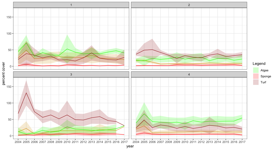
We rename the result to a descriptive object and write it to outputs/.
benthicOrganismCommunityCluster <- nmds_coordinates
write.csv(
  benthicOrganismCommunityCluster,
  mkfilefn(benthicOrganismCommunityCluster),
  row.names = F
)
We describe the whole data frame in *_dfdesc.
benthicOrganismCommunityCluster_dfdesc <-
  "data from multivariate community clustering of sites based on benthic surveys of coral, algae, sponge, turf, and non-living components between 2007 and 2017. Includes TCRMP and VINPS sites that contained this level of detail."
We describe each column in *_desc.
benthicOrganismCommunityCluster_desc <- make_desc(benthicOrganismCommunityCluster)
#View(tempDat_yearly_desc)
benthicOrganismCommunityCluster_desc$description <- c(
  "NMDS axis 1 coordinate",
  "NMDS axis 2 coordinate",
  "survey site",
  "survey year",
  "cluster as determined by kmeans clustering of mean values for each site (each site only belongs to 1 cluster)",
  "depth",
  "cluster/site named variable",
  "coral percent cover (averaged across replicates)",
  "algae percent cover (averaged across replicates)",
  "sponge percent cover (averaged across replicates)",
  "turf percent cover (averaged across replicates)",
  "nonliving percent cover (averaged across replicates)",
  "monitoring program"
)
We write the metadata sidecar alongside the data file.
summary_text <- summarize_data_frame(benthicOrganismCommunityCluster, benthicOrganismCommunityCluster_dfdesc,benthicOrganismCommunityCluster_desc)
file_conn <- file(mkmetafilefn(benthicOrganismCommunityCluster), "w")
writeLines(summary_text, file_conn)
close(file_conn)The clustered community data and its metadata are generated by the chunks above and offered below.
s5pt3_benthicOrganismCommunityCluster_40sites_2004_2017.csvs5pt3_benthicOrganismCommunityCluster_40sites_2004_2017.txtversion 1.0.0 • in-review • data ≤ 2023-12-31