Reef Code

About Analyses Outputs

About this site

Data Sources

more about

study sites making of the logo

benthic cover

about 2.1 Reformat raw benthic cover data 2.2 Cross-reference benthic codes 2.3 percentage cover of main benthic categories 2.4 percentage cover of coral genera 2.5 percentage cover of coral species 2.6 percentage cover of coral trait groups 2.7 percentage cover of algae taxa 2.8 percentage cover of sponge morphs 2.9 percentage cover of zoanthids and gorgonians 2.10 percentage cover of other benthic categories

internal drivers

3.1 coral health 3.2 coral interactions 3.3 fish biodiversity 3.3b fish biodiversity using NOAA data 3.4 herbivory 3.5 coral biodiversity 3.6 diadema 3.7 nuisance species

external drivers

4.1 site rugosity 4.2 site depth 4.3 site distances from shore 4.4 daily temperatures 4.5 monthly and annual DHW and temperature 4.6 currents 4.7 management 4.8 wave benthic orbital velocities pt 1 4.9 wave benthic orbital velocities pt 2 4.10 water quality 4.11 sedimentation 4.12 connectivity

resilience values

5.1 absolute and relative coral cover and diversity 5.2 resilience classification based on coral cover 5.3 benthic community: benthic organisms 5.4 NMDS of coral genera during recovery period

Reproductive Mode & RarityOlinger et al., In Review

Overview TCRMP VINPS CSUN Octocorals Interactive

2023, 2024 Bleaching EventOlinger et al. In Prep

VI Reef Resilience StudyOlinger et al. Coming Soon

(Any Others?)co-author suggestions welcome

2.4 Percentage cover of coral genera

2.4 Percentage cover of coral genera

On this page

This page aggregates surveyed coral species into genera and computes annual percent cover of each genus at every monitoring site. It produces the site-faceted stacked-area figure Figure 1 and a downloadable long-format table of genus-level cover. Grouping corals at the genus level follows the genera groupings in the CSUN random data, the genus-level resilience scores of Van Woesik et al. (2012), and the genus-frequency analysis of Moritz et al. (2021). The genus-level table is a data product that downstream resilience and biodiversity pages read, so the numbers here feed the rest of the site.

Data sources

This page reads the cross-referenced benthic workspace written by section 2.2, which combines the three monitoring programs TCRMP, VINPS, and CSUN into per-program cover matrices (tcrmp_benthicDat, vinps_benthicDat, csun_random_benthicDat) plus the benthic-code cross-reference (benthicCodes). Site metadata (sitedat) supplies the depth used to order facets from shallow to deep. The genus grouping keeps only coral rows and combines the three programs into one long-format cover table, offered below in the Download the data section.

WarningSampling differs by program

The three programs do not share a sampling design, so their cover series are not directly comparable point-for-point. TCRMP and VINPS use replicate transects, so their annual site cover is transect-averaged and carries a standard error. CSUN records no transect replicate, so its cover is computed cumulatively at each site and shows no error bar. The programs also start in different years. Read the black points and error bars in Figure 1 with these differences in mind.

Load workspace and define variables

The reformatted cover data and the benthic-code cross-reference come from the section 2.2 output.

load("benthicCoverXrefBenthicCodes.RData")

groupingvar names the grouping used on this page (coral genera), and section sets the output-file prefix (s2pt4).

# subfoldername <- "benthicCoverGrouped"
groupingvar <- "coralGenera"
section <- "s2pt4" # for naming

Reorganize benthicDat into genus subgroups

NoteWhat happens here

Two functions do the regrouping. getBenthicDatColInds() finds, for each genus, which columns of a program’s cover matrix belong to it. makeGroupedBenthicDat() then sums those columns into one column per genus. The pattern runs once per program (TCRMP, VINPS, CSUN), and the three results merge into one long table.

Restrict the cross-reference to coral rows so only corals are grouped into genera.

benthicCodes$tcrmp_trait[which(benthicCodes$csun_random_code == "Millepora")] <-
  NA
benthicCodes <- benthicCodes[which(benthicCodes$tcrmp_Category=="Coral"),]

getBenthicDatColInds()

This is one of two functions that connect benthicDat to benthicCodes for all three programs.

getBenthicDatColInds() makes _columnInds that stores column indices of benthic codes corresponding to each item of coralGenera

arguments:

• benthicDat is benthic dataset of interest

• codecolumn is the name of the column of benthic code containing the code for benthicdat

• groupingcolumn is the name of the column of benthic codes where the grouping variable of interest is stored.

getBenthicDatColInds <-
  function(benthicDat, codecolumn, groupingcolumn) {
    codecolind <-
      which(colnames(benthicCodes) == codecolumn)
    groupingcolind <-
      which(colnames(benthicCodes) == groupingcolumn)
    genusdf <-
      data.frame(group =
                   unique(benthicCodes[, groupingcolind]),
                 colinds =
                   rep(0, length(unique(benthicCodes[, groupingcolind]))))
    for (i in 1:nrow(genusdf)) {
      codei <-
        benthicCodes[which(benthicCodes[, groupingcolind] == genusdf$group[i]), ]
      genusdf$colinds[i] <-
        list(which(colnames(benthicDat) %in% codei[, codecolind]))
    }
    # UAGA-guard: warn on benthicDat data columns whose code is absent from benthicCodes and is
    # therefore silently dropped (the footgun that lost VINPS Agaricia agaricites, code UAGA).
    .known <- benthicCodes[[codecolind]]; .known <- .known[nchar(.known) > 0]
    .meta_cols <- c("program","date","site","period","replicate","replicatetype","nopts",
                    "Year","Date","SiteFullName","year","month","percentCover_allCoral",
                    "PC","Check","Notes","Transect")
    .dropped <- setdiff(colnames(benthicDat), c(.known, .meta_cols))
    if (length(.dropped) > 0)
      warning("getBenthicDatColInds(", codecolumn, "): ", length(.dropped),
              " data column(s) have codes absent from benthicCodes and are DROPPED: ",
              paste(.dropped, collapse = ", "), " -- add them to benthicCodes if they are taxa.")
    return(genusdf)
  }

Apply getBenthicDatColInds() to each program’s cover matrix.

tcrmp_columnInds <-
  getBenthicDatColInds(tcrmp_benthicDat, "tcrmp_Code", "genus")
vinps_columnInds <-
  getBenthicDatColInds(vinps_benthicDat, "vinps_TaxonCode", "genus")
csunrandom_columnInds <-
  getBenthicDatColInds(csun_random_benthicDat, "csun_random_code", "genus")

The TCRMP mapping resolves 29 genus groups and the CSUN random mapping resolves 29. Table 1 previews the TCRMP genus-to-column map.

kbl(tcrmp_columnInds) |>
  kable_paper(full_width = F) |>
  kable_styling(
    fixed_thead = T,
    bootstrap_options = c("hover", "condensed"),
    font_size = 8
  ) |>
  scroll_box(width = "100%", height = "250px")

Sec 2.4 Table 1: TCRMP genus groups and the cover-matrix column indices assigned to each (preview of tcrmp_columnInds).

group	colinds
Millepora	38, 39, 40
Dendrogyra	22
Acropora	9, 15, 16
Orbicella	46, 48, 49, 50
Scolymia	61, 62, 65
Porites	51, 52, 53, 56, 57, 58
Mycetophyllia	31, 36, 37, 41, 45
Mussa	32
Madracis	30, 35, 42
Isopyhyllastrea	28
unknown	20
unknown juv.	21
Helioseris	27
Oculina	47
Solenastrea	60, 63
Tubastraea	69
Stephanocoenia	64
Siderastrea	66, 67, 68
Montastraea	34, 44
Meandrina	43
Favia	26
Eusmilia	25
Diploria	23
Dichocoenia	24
Colpophyllia	19
Pseudodiploria	55, 59
Manicina	33
Agaricia	8, 10, 11, 12, 13, 14, 17, 18
Isophyllia	29

Drop the CSUN genus groups that resolve to no column, since not every genus is present in the CSUN random data.

csunrandom_columnInds$colinds[sapply(csunrandom_columnInds$colinds, function(x) length(x) == 0L)] <- NA
csunrandom_columnInds$colinds <-
  unlist(csunrandom_columnInds$colinds)
csunrandom_columnInds <-
  csunrandom_columnInds[-which(is.na(csunrandom_columnInds$colinds)),]
csunrandom_columnInds <-
  csunrandom_columnInds |> filter(group != "Millepora")

makeGroupedBenthicDat()

This is the second function that connects benthicDat to benthicCodes for all three programs.

makeGroupedBenthicDat() extracts the column indices (colinds) from each row of *_columnInds.

If only one index in colinds , assigns the corresponding column from benthicdat to the i-th column of a data frame _groupedBenthicDat.

if more than one index in colinds, stores row sum of benthicDat[,colinds] in the i-th column of _groupedBenthicDat.

arguments:

• benthicDat is benthic dataset of interest

• columnInds is the output of getBenthicDatColInds() above that contains column indices of benthic codes for each benthic subgroup of interest

makeGroupedBenthicDat <- function(benthicDat, columnInds) {
  groupeddat <- data.frame(matrix(nrow = nrow(benthicDat),
                                  ncol = nrow(columnInds)))
  colnames(groupeddat) <- columnInds$group
  benthicDat <- benthicDat %>% dplyr::mutate(dplyr::across(dplyr::where(is.numeric), ~replace(.x, is.na(.x), 0))) 
  for (i in 1:nrow(columnInds)) {
    geni <- columnInds[i,]
    datcoli <- unlist(geni$colinds)
    if (length(datcoli) == 1) {
      groupeddat[, i] <- benthicDat[, datcoli]
    } else {
      groupeddat[, i] <- rowSums(benthicDat[, datcoli])
    }
  }
  groupeddat <- cbind(benthicDat[, 1:6], groupeddat)
  return(groupeddat)
}

Apply makeGroupedBenthicDat() to each program’s cover matrix and its column-index map.

tcrmp_groupedBenthicDat <-
  makeGroupedBenthicDat(tcrmp_benthicDat, tcrmp_columnInds)
vinps_groupedBenthicDat <-
  makeGroupedBenthicDat(vinps_benthicDat, vinps_columnInds)
csun_groupedBenthicDat <-
  makeGroupedBenthicDat(csun_random_benthicDat, csunrandom_columnInds)

Table 2 previews the first rows of the TCRMP genus-grouped table: the six survey identifier columns followed by one column per coral genus.

kbl(head(tcrmp_groupedBenthicDat)) |>
  kable_paper(full_width = F) |>
  kable_styling(
    fixed_thead = T,
    bootstrap_options = c("hover", "condensed"),
    font_size = 8
  ) |>
  scroll_box(width = "100%", height = "250px")

Sec 2.4 Table 2: First rows of tcrmp_groupedBenthicDat: survey identifiers plus one percent-cover column per coral genus.

program	date	site	period	replicate	replicatetype	Millepora	Dendrogyra	Acropora	Orbicella	Scolymia	Porites	Mycetophyllia	Mussa	Madracis	Isopyhyllastrea	unknown	unknown juv.	Helioseris	Oculina	Solenastrea	Tubastraea	Stephanocoenia	Siderastrea	Montastraea	Meandrina	Favia	Eusmilia	Diploria	Dichocoenia	Colpophyllia	Pseudodiploria	Manicina	Agaricia	Isophyllia
TCRMP	2001-04-25	Cane Bay	Annual	1	transect	0.00	0	0	1.15	0	2.30	0.00	0	0	0	0.00	0	0	0	0	0	0.00	0.00	1.53	0	0	0	0.00	0	0.00	0.00	0	0.00	0.00
TCRMP	2001-04-25	Cane Bay	Annual	2	transect	0.00	0	0	12.11	0	4.29	0.00	0	0	0	0.78	0	0	0	0	0	0.00	0.00	5.86	0	0	0	2.34	0	0.39	0.00	0	1.17	0.00
TCRMP	2001-04-25	Cane Bay	Annual	3	transect	0.00	0	0	22.09	0	6.21	0.39	0	0	0	0.78	0	0	0	0	0	0.00	1.94	2.71	0	0	0	0.00	0	0.78	0.39	0	1.55	0.39
TCRMP	2001-04-25	Cane Bay	Annual	4	transect	0.00	0	0	21.38	0	1.81	1.45	0	0	0	0.36	0	0	0	0	0	0.00	0.00	5.07	0	0	0	0.00	0	0.00	0.00	0	0.72	0.00
TCRMP	2001-04-25	Cane Bay	Annual	5	transect	0.00	0	0	17.72	0	0.39	0.00	0	0	0	0.39	0	0	0	0	0	0.00	3.54	0.00	0	0	0	0.00	0	0.00	0.00	0	1.18	0.00
TCRMP	2001-04-25	Cane Bay	Annual	6	transect	0.38	0	0	9.02	0	4.14	0.38	0	0	0	0.38	0	0	0	0	0	0.38	0.38	1.13	0	0	0	0.00	0	0.00	0.38	0	0.38	0.00

Merge the three programs

The three _groupedBenthicDat tables hold different sets of genera, because some genera never appear in the CSUN data. The steps below give every table the same columns, stack them, then reshape to long format.

Collect every genus column that appears in any program.

all_columns <-
  unique(c(
    colnames(tcrmp_groupedBenthicDat),
    colnames(vinps_groupedBenthicDat),
    colnames(csun_groupedBenthicDat)
  ))

Identify the genus columns missing from each program.

missing_columns_tcrmp <-
  setdiff(all_columns, colnames(tcrmp_groupedBenthicDat))
missing_columns_vinps <-
  setdiff(all_columns, colnames(vinps_groupedBenthicDat))
missing_columns_csung <-
  setdiff(all_columns, colnames(csun_groupedBenthicDat))

Add each missing genus column as NA.

for (col in missing_columns_tcrmp) {
  tcrmp_groupedBenthicDat[[col]] <- NA
}
for (col in missing_columns_vinps) {
  vinps_groupedBenthicDat[[col]] <- NA
}
for (col in missing_columns_csung) {
  csun_groupedBenthicDat[[col]] <- NA
}

Reorder every table to the shared column order.

tcrmp_groupedBenthicDat <- tcrmp_groupedBenthicDat[, all_columns]
vinps_groupedBenthicDat <- vinps_groupedBenthicDat[, all_columns]
csun_groupedBenthicDat <- csun_groupedBenthicDat[, all_columns]

Stack the three tables into one groupedBenthicDat.

groupedBenthicDat <-
  rbind(tcrmp_groupedBenthicDat,
        vinps_groupedBenthicDat,
        csun_groupedBenthicDat)

Add a year column derived from the survey date.

groupedBenthicDat <-
  cbind(year = lubridate::year(groupedBenthicDat$date),
        groupedBenthicDat)

Reshape from one column per genus to one row per genus (long format), and drop rows with no cover value.

groupedBenthicDat <- groupedBenthicDat |>
  tidyr::gather(!!groupingvar, "perccover", 8:ncol(groupedBenthicDat))

groupedBenthicDat <- groupedBenthicDat |>
  filter(!is.na(perccover))

Flag each row as present (pres = 1) or absent (pres = 0) for the genus.

groupedBenthicDat$pres <- rep(0, nrow(groupedBenthicDat))
groupedBenthicDat$pres[groupedBenthicDat$perccover > 0] <- 1

Summarize and plot

For TCRMP and VINPS, the summary is annual transect-averaged percent cover of coral genera at each site, with a standard error from the transect replicates. For CSUN, the summary is cumulative percent cover of coral genera at each site, because CSUN has no transect replicate to average over.

Annual total coral cover per site

Sum genus cover within each transect, then average across transects to get annual total coral cover and its standard error at each site.

totaldatCovSum <- groupedBenthicDat |>
  dplyr::group_by(year, date, program, site, period, replicate) |>
  dplyr::summarise(perccover = sum(perccover))

totaldatCovSum <- totaldatCovSum |>
  dplyr::group_by(year, date, program, site) |>
  dplyr::summarise(
    meancov = mean(perccover),
    sdcov = sd(perccover),
    secov = sd(perccover) / (sqrt(length(perccover))),
    n = length(perccover)
  )

totaldatCovSum <- totaldatCovSum %>% dplyr::mutate(dplyr::across(dplyr::where(is.numeric), ~replace(.x, is.na(.x), 0)))

Annual cover per genus per site

Summarize annual percent cover for each individual genus at each site.

groupedBenthicDatCovSum <- groupedBenthicDat |>
  dplyr::group_by(year, date, program, site, period, coralGenera) |>
  dplyr::summarise(
    meancov = mean(perccover),
    sdcov = sd(perccover),
    secov = sd(perccover) / (sqrt(length(perccover))),
    n = length(perccover)
  )
groupedBenthicDatCovSum <- groupedBenthicDatCovSum %>% dplyr::mutate(dplyr::across(dplyr::where(is.numeric), ~replace(.x, is.na(.x), 0)))

Genus-cover figure

Figure 1 stacks each genus’s cover over time, one panel per site ordered shallow to deep, with total coral cover overlaid as black points and a dashed 2005 bleaching reference line. Reading down a column of panels shows how the genus makeup of coral cover shifts with depth and over time.

#add site info so can plot according to increasing depth
groupedBenthicDatCovSum <-
  merge(groupedBenthicDatCovSum, sitedat, by = "site")
groupedBenthicDatCovSum <-
  groupedBenthicDatCovSum[order(groupedBenthicDatCovSum$depth), ]
groupedBenthicDatCovSum$site <- factor(groupedBenthicDatCovSum$site,
                                       levels = unique(groupedBenthicDatCovSum$site))

#add site info so can plot according to increasing depth
totaldatCovSum <-
  merge(totaldatCovSum, sitedat, by = "site")
totaldatCovSum <-
  totaldatCovSum[order(totaldatCovSum$depth), ]
totaldatCovSum$site <- factor(totaldatCovSum$site,
                              levels = unique(totaldatCovSum$site))

create_stacked_area_plot <- function(data_stacked, data_total, 
                                     x_var = "year", y_var = "meancov", 
                                     fill_var = "coralGenera", facet_var = "site",
                                     error_var = "secov",
                                     min_year = NULL, max_year = NULL,
                                     highlight_year = NULL,
                                     max_facets_per_page = 35) {
  
  # Determine x-axis limits if not provided
  if (is.null(min_year)) min_year <- floor(min(data_stacked[[x_var]]))
  if (is.null(max_year)) max_year <- ceiling(max(data_stacked[[x_var]]))
  
  # Calculate optimal number of rows and columns
  n_facets <- length(unique(data_stacked[[facet_var]]))
  n_facets <- min(n_facets, max_facets_per_page)  # Limit to max_facets_per_page
  n_col <- ceiling(sqrt(n_facets))
  n_row <- ceiling(n_facets / n_col)
  
  # Create base plot
  p <- ggplot() +
    geom_area(data = data_stacked,
              aes(x = .data[[x_var]], y = .data[[y_var]], fill = .data[[fill_var]]),
              position = 'stack') +
    geom_point(
      data = data_total,
      aes(x = .data[[x_var]], y = .data[[y_var]]),
      color = "black",
      size = 0.5
    ) +
    geom_linerange(
      data = data_total,
      aes(
        x = .data[[x_var]],
        ymin = .data[[y_var]] - .data[[error_var]],
        ymax = .data[[y_var]] + .data[[error_var]]
      ),
      color = "black",
      linewidth = 0.5
    ) +
    facet_wrap(vars(.data[[facet_var]]), nrow = n_row, ncol = n_col, scales = "free_x") +
    labs(y = "Percent cover", x = toupper(x_var)) +
    scale_y_continuous(expand = c(0, 0)) +
    scale_x_continuous(
      expand = expansion(mult = 0.04),
      breaks = seq(min_year, max_year, by = 1),
      labels = function(x) ifelse(x %% 5 == 0, paste0("'", substr(x, 3, 4)), "")
    ) +
    theme_bw() +
    theme(
      strip.text = element_text(size = 10),
      legend.position = "bottom",
      panel.grid = element_blank()
    )
  
  # Add highlight line if specified
  if (!is.null(highlight_year)) {
    p <- p + geom_vline(
      xintercept = highlight_year,
      color = "gray50",
      alpha = 0.5,
      linetype = "dashed"
    )
  }
  
  return(p)
}

# Usage example:
stack <- create_stacked_area_plot(
  data_stacked = groupedBenthicDatCovSum,
  # x_var = "date", # default is year
  data_total = totaldatCovSum,
  min_year = minyear,
  max_year = maxyear,
  highlight_year = 2005,
  fill_var = "coralGenera",
  max_facets_per_page = length(unique(groupedBenthicDatCovSum$site))
)

# Display the plot
print(stack)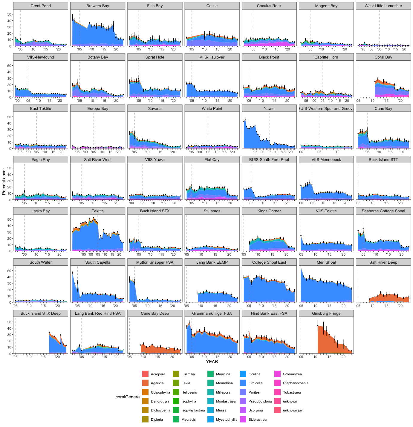

Sec 2.4 Figure 1: Percent cover of coral over time at each site, separated into genera. Sites are ordered shallow to deep. Black points show average total coral cover ± SE (TCRMP and VINPS transect replicates; CSUN cumulative, no error bar). The dashed line marks the 2005 bleaching event.

TipKey result

Figure 1 shows the genus makeup of coral cover through time at every monitored site, ordered shallow to deep. The stacked bands separate the genera that drive a site’s total cover (the black points), so shifts in which genera dominate after disturbance, and differences between shallow and deep sites, are visible directly. This genus-level table is the input for the coral-genera resilience and ordination analyses later on the site.

• Derived data: s2pt4_benthicCoverCoralGenera_49sites_1987_2023.csv (16.9 MB)

• Metadata: s2pt4_benthicCoverCoralGenera_49sites_1987_2023.txt

---

version 1.0.0 • in-review • data ≤ 2023

References

Moritz, C., Simon J. Brandl, H. Rouzé, J. Vii, Gonzalo Perez-Rosales, P. Bosserelle, Y. Chancerelle, et al. 2021. “Long-Term Monitoring of Benthic Communities Reveals Spatial Determinants of Disturbance and Recovery Dynamics on Coral Reefs.” https://doi.org/10.3354/MEPS13807.

Van Woesik, Robert, Erik C. Franklin, Jennifer O’Leary, Tim R. McClanahan, James S. Klaus, and Ann F. Budd. 2012. “Hosts of the Plio-Pleistocene Past Reflect Modern-Day Coral Vulnerability.” Proceedings of the Royal Society B: Biological Sciences 279 (1737): 2448–56. https://doi.org/10.1098/rspb.2011.2621.