Reef Code

about 2.1 Reformat raw benthic cover data 2.2 Cross-reference benthic codes 2.3 percentage cover of main benthic categories 2.4 percentage cover of coral genera 2.5 percentage cover of coral species 2.6 percentage cover of coral trait groups 2.7 percentage cover of algae taxa 2.8 percentage cover of sponge morphs 2.9 percentage cover of zoanthids and gorgonians 2.10 percentage cover of other benthic categories

internal drivers

3.1 coral health 3.2 coral interactions 3.3 fish biodiversity 3.3b fish biodiversity using NOAA data 3.4 herbivory 3.5 coral biodiversity 3.6 diadema 3.7 nuisance species

external drivers

4.1 site rugosity 4.2 site depth 4.3 site distances from shore 4.4 daily temperatures 4.5 monthly and annual DHW and temperature 4.6 currents 4.7 management 4.8 wave benthic orbital velocities pt 1 4.9 wave benthic orbital velocities pt 2 4.10 water quality 4.11 sedimentation 4.12 connectivity

resilience values

5.1 absolute and relative coral cover and diversity 5.2 resilience classification based on coral cover 5.3 benthic community: benthic organisms 5.4 NMDS of coral genera during recovery period

Reproductive Mode & RarityOlinger et al., In Review

Overview TCRMP VINPS CSUN Octocorals Interactive

2023, 2024 Bleaching EventOlinger et al. In Prep

VI Reef Resilience StudyOlinger et al. Coming Soon

(Any Others?)co-author suggestions welcome

4.8 Wave benthic orbital velocities pt 1

Last updated

July 6, 2026

4.8 Wave benthic orbital velocities pt 1

This page is part 1 of a two-part wave series. It extracts significant wave height (Hsig) and wave period (Per) from pre-downloaded slices of the SWAN aggregation model, reading each biweekly netCDF slice and isolating the grid cells whose latitude and longitude pairs match the 50 USVI reef sites. It writes the extracted Hsig and Per series to CSV, plots both time series as a visual check that the extraction produced continuous, sensible wave signals, and produces a site-to-grid-coordinate lookup. Part 2 (4.9) reads these CSVs and computes benthic orbital velocities (BOVs) for each site.

Data sources

This page uses the SWAN wave model slices (biweekly Hsig/Per netCDF grids) together with a reference site catalog carrying the grid coordinate determined for each of the 50 sites. From these inputs it derives a per-coordinate Hsig/Per time-series product and a site-to-grid-coordinate lookup, both offered in the Downloads section below.

Import data

We load the master catalog of 50 USVI reef sites into sitedat. This catalog comes from the waves subfolder because it carries the grid coordinate we determined for each site in an earlier version of this analysis.

Show code

# sitedat <- read.csv("../../../RRSdata/00_RRS_dataCatalogStatus/00_RRS_siteMaster_allSites_data.csv")
# metadat <- readLines("../../../RRSdata/00_RRS_dataCatalogStatus/00_RRS_siteMaster_allSites_metadata.txt")

sitedat <- read.csv(
  "../../../RRSdata/data_adhoc/waves/referenceSitedatWithGridCoords/s4pt9_bov_summary_statistics_50sites_2015_2015.csv"
)

metadat <- readLines(
  "../../../RRSdata/data_adhoc/waves/referenceSitedatWithGridCoords/s4pt9_bov_summary_statistics_50sites_2015_2015.txt"
)

List the raw netCDF files

We collect the full paths to the biweekly SWAN netCDF slices that the extraction function reads below.

Show code

file_names <- list.files(
  "../../../RRSdata/data_adhoc/waves/SWANHsigPer_wholeGrid_biweekly_ncs",
  full.names = TRUE
)

Define the extraction function

What happens here: nc_to_csv() opens one netCDF slice, matches its grid latitudes and longitudes to the site coordinates in sitedat, reads the Hsig and Per series at each matched cell, and returns a tidy data frame of time, Hsig, and Per per site coordinate.

Show code

nc_to_csv <- function(file, sitedat) {
  # Import netcdf data
  nc <- nc_open(file)
  
  # Read the entire time array
  time <- ncvar_get(nc, 'time')
  latitudes <- ncvar_get(nc, 'latitude')
  longitudes <- ncvar_get(nc, 'longitude')
  
  # Convert time from seconds since 1970-01-01 to POSIXct
  time <- as.POSIXct(time, origin = "1970-01-01", tz = "UTC")
  
  # Function to find indices of matching lat/lon values
  find_indices <- function(values, target_values) {
    diff_matrix <- outer(
      values,
      target_values,
      FUN = function(x, y)
        abs(x - y)
    )
    matching_matrix <- diff_matrix < 1e-10
    apply(matching_matrix, 2, which)
  }
  
  latIndex <- find_indices(latitudes, sitedat$gridLat)
  lonIndex <- find_indices(longitudes, sitedat$gridLon)
  
  # Create a dataframe of lat and lon index pairs from sitedat$gridLat and sitedat$gridLon
  sitedat <- sitedat %>% mutate(site_coord = paste(round(gridLat, 2), round(gridLon, 2), sep = "_"))
  
  # Create the combinations dataframe
  combinations <- data.frame(lat = latitudes[latIndex], lon = longitudes[lonIndex]) %>%
    mutate(site_coord = paste(round(lat, 2), round(lon, 2), sep = "_")) %>%
    filter(site_coord %in% sitedat$site_coord) %>%
    distinct(site_coord, .keep_all = TRUE) %>%
    mutate(latIn = latIndex[match(lat, lat)], lonIn = lonIndex[match(lon, lon)]) %>%
    arrange(site_coord)
  
  sitedat <- sitedat %>% arrange(site_coord)
  
  # Read slices of Hsig and Per data at each lat and lon index pair
  data_list <- apply(combinations, 1, function(x) {
    latIn <- as.numeric(x['latIn'])
    lonIn <- as.numeric(x['lonIn'])
    
    hsig_data <- ncvar_get(nc,
                           'Hsig',
                           start = c(lonIn, latIn, 1),
                           count = c(1, 1, -1))
    per_data <- ncvar_get(nc,
                          'Per',
                          start = c(lonIn, latIn, 1),
                          count = c(1, 1, -1))
    
    list(
      site_coord = x['site_coord'],
      time = time,
      hsig_data = hsig_data,
      per_data = per_data
    )
  })
  
  # Flatten the data list into a data frame
  flattened_data <- do.call(rbind, lapply(data_list, function(item) {
    data.frame(
      site_coord = rep(item$site_coord, length(item$hsig_data)),
      time = item$time,
      hsig = item$hsig_data,
      per = item$per_data
    )
  }))
  
  # Format the time to include the midnight hour
  flattened_data$time <- format(flattened_data$time, "%m/%d/%Y %H:%M:%S")
  nc_close(nc)
  return(flattened_data)
}

Run the extraction

We apply nc_to_csv() to every netCDF slice and stack the results into swanHsigPerDat, then derive the date range for the output file name.

Show code

swanHsigPerDat <- nc_to_csv(file_names[1], sitedat)

for (i in 2:length(file_names)) {
  swanHsigPerDat <- rbind(swanHsigPerDat, nc_to_csv(file_names[i], sitedat))
}

min_date <-
  format(min(as.POSIXct(swanHsigPerDat$time, format = "%m/%d/%Y %H:%M:%S")), "%Y%m%d")
max_date <-
  format(max(as.POSIXct(swanHsigPerDat$time, format = "%m/%d/%Y %H:%M:%S")), "%Y%m%d")

# Construct the file name
file_base_name <-
  paste0(section,
         "_SWANHsigPer_AllSiteCoords_",
         min_date,
         "_",
         max_date)
csv_file_name <- paste0(file_base_name, ".csv")
metadata_file_name <- paste0(file_base_name, ".txt")

Build the wave series figures

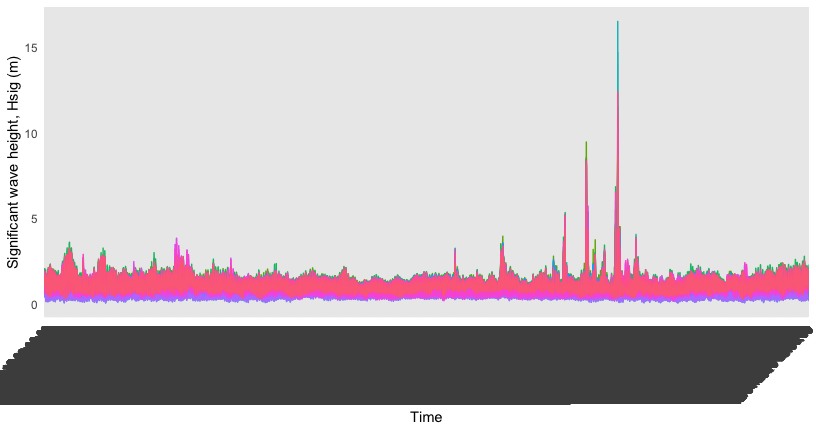
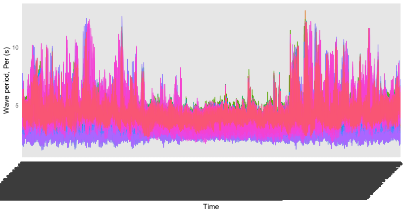
We build one time-series figure for significant wave height and one for wave period. Each line is a site coordinate pair; the legend is suppressed because the 50 overlapping series read as a signal envelope rather than as individually identifiable sites.

Show code

p <-
  ggplot(swanHsigPerDat, aes(x = time, y = hsig, color = site_coord)) +
  geom_line(aes(group = site_coord)) +
  labs(x = "Time", y = "Significant wave height, Hsig (m)") +
  # scale_x_date(date_labels = "%Y", date_breaks = "1 year") +
  theme_minimal(base_size = 11) +
  theme(legend.position = "none",
        axis.text.x = element_text(angle = 45, hjust = 1),
        panel.grid.minor = element_blank())


p2 <-
  ggplot(swanHsigPerDat, aes(x = time, y = per, color = site_coord)) +
  geom_line(aes(group = site_coord)) +
  labs(x = "Time", y = "Wave period, Per (s)") +
  theme_minimal(base_size = 11) +
  theme(legend.position = "none",
        axis.text.x = element_text(angle = 45, hjust = 1),
        panel.grid.minor = element_blank())

Wave time series

Figure 1 shows significant wave height and Figure 2 shows wave period, each plotted across all 50 site coordinate pairs for the extracted date range. Both series should read as continuous, well-behaved wave signals; that is the check this page performs before part 2 (4.9) converts them into benthic orbital velocities.

Show code

Sec 4.8 Figure 1: Significant wave height (Hsig, m) over time. Each line is one site coordinate pair (50 pairs across the 50 USVI reef sites).

Show code

p2

Sec 4.8 Figure 2: Wave period (Per, s) over time. Each line is one site coordinate pair (50 pairs across the 50 USVI reef sites).

Downloads

The buttons below download the extracted Hsig/Per series, the site-to-coordinate lookup, and the metadata for each, all generated from the objects built above.

version 1.0.0 • in-review • data ≤ 2023-12-31

4.8 Wave benthic orbital velocities pt 1

On this page

Data sources

Import data

List the raw netCDF files

Define the extraction function

Run the extraction

Build the wave series figures

Wave time series

Downloads