Show code
sitedat <-
  read.csv(
    "../../../RRSdata/00_RRS_dataCatalogStatus/00_RRS_siteMaster_allSites_data.csv"
)This page attaches marine-management attributes to each VIRRS monitoring site. We assigned every site to its overlapping managed area by hand: we opened the USA Dataset of Marine Managed Areas in the online map viewer, imported the VIRRS study sites, and read off the managed area each site falls within. The page reads three tables (the site master, the managed-area catalog, and the manual site-to-area assignments), joins them into one site-management table, and classifies each site into four levels of fishing protection, following the fishing-gear-restriction scheme of Gove et al. (2023). It produces one downloadable product, siteManagementStatus, with its metadata sidecar, plus a figure (Figure 1) that maps the protection levels across the study region.
This page uses the management datasets: the site master (program, site, latitude, longitude), the managed-area catalog (managed-area attributes from the USA Dataset of Marine Managed Areas), and the manual site-to-area assignments. Each links to its entry on the Data Sources page. The derived site-management table produced here is available in the Downloads section below.
This table holds the program, site name, and coordinates for every monitoring site.
sitedat <-
read.csv(
"../../../RRSdata/00_RRS_dataCatalogStatus/00_RRS_siteMaster_allSites_data.csv"
)This table catalogs the marine managed areas and their attributes.
managedAreas <-
  read.csv(
    "../../../RRSdata/data_adhoc/management/marineManagedAreas_data.csv"
)This table records the managed area we hand-assigned to each site.
managedAreaAssignments <-
  read.csv(
    "../../../RRSdata/data_adhoc/management/marineManagedAreas_siteAssignments_allSites_data.csv"
)We join the manual assignments to the managed-area catalog and to the site master, then rename the columns to a compact, descriptive set.
siteManagement <- managedAreaAssignments |>
  left_join(managedAreas, by = "Site.Name") |>
  select(-c(OBJECTID, Site.ID, Country, State))

siteManagement <- siteManagement[, c(1:24)]

siteManagement <- siteManagement |>
  select(
    -c(
      Effective.From,
      Effective.To,
      Season,
      Report.Violations,
      S.57.Category,
      IUCN.Category,
      WDPA.ID
    )
  )

siteManagement <- siteManagement |>
  left_join(sitedat |> select(c(program, site, lat, lon)), by = "site") |>
  select(program, site, lat, lon, everything())

colnames(siteManagement) <-
  c(
    "program",
    "site",
    "lat",
    "lon",
    "managedAreaName",
    "website",
    "managingAuthority",
    "levelOfGovernment",
    "designation",
    "categories",
    "yearEstablished",
    "purpose",
    "restrictions",
    "allowed",
    "regulationName",
    "regulationWebsite",
    "latestUpdates",
    "protectionFocus",
    "speciesOfConcern",
    "levelFishingProtection"
)We classify each site into one of four levels of fishing protection, then map those levels across the study region. Figure 1 shows where the more- and less-protected sites sit, which lets downstream analyses group sites by protection level.
siteManagement$LFP <- "Least Restrictive"
siteManagement$LFP[grep("Heavily", siteManagement$levelFishingProtection)] <-
  "Heavily Restrictive"
siteManagement$LFP[grep("Moderately", siteManagement$levelFishingProtection)] <-
  "Moderately Restrictive"
siteManagement$LFP[grep("Most ", siteManagement$levelFishingProtection)] <-
  "Most Restrictive"

siteManagement$LFP <-
  factor(
    siteManagement$LFP,
    levels = c(
      "Least Restrictive",
      "Moderately Restrictive",
      "Heavily Restrictive",
      "Most Restrictive"
    )
  )

# Define the bounding box
bbox <- make_bbox(siteManagement$lon, siteManagement$lat, f = 0.1)

# Fetch the map
# map <-
#   get_map(location = bbox,
#           source = "stamen",
#           maptype = "toner-lite")  # You can change the source if you prefer a different map style

background_map <-
  st_read(dsn = "../shapefiles/pvishrpl/", layer = "pvishrpl", quiet = TRUE)
lon_range <- range(sitedat$lon)
lat_range <- range(sitedat$lat)


p <- ggplot() +
  # Plot the background map
  geom_sf(data = background_map, fill = "grey50", color = "white") +
  geom_point(
    data = siteManagement,
    aes(x = lon, y = lat, fill = LFP),
    shape = 21,
    col = "black",
    size = 4,
    alpha = 0.7
  ) +
  geom_point() +
  labs(x = "Longitude", y = "Latitude") +
  scale_fill_manual(values = c("blue", "green", "orange", "red")) +
  theme(axis.text.x = element_text(angle = 45, hjust = 1)) +
  theme(legend.position = "bottom") +
  coord_sf(xlim = lon_range, ylim = lat_range) +
  # labs(x = "Longitude", y = "Latitude") +
  theme_minimal() +
  theme(legend.position = "bottom")

p
# svg(filename="management.svg", width = 13, height =13)
# p
# dev.off()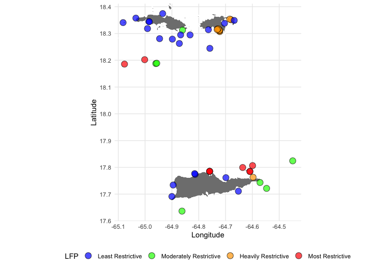
We keep only sites added by the maxyearadded cutoff, so the management table matches the site set used across the rest of the analysis.
The buttons below download the site-management table and its metadata sidecar, both generated by the code on this page.
s4pt7_siteManagementStatus_43sites.csvs4pt7_siteManagementStatus_43sites.txtversion 1.0.0 • in-review • data ≤ 2023-12-31