3.2 Coral interactions

Last updated

July 6, 2026

3.2 Coral interactions

On this page

This page processes the coral interaction records from TCRMP coral health surveys and summarizes how often corals interact with other organisms and how much of each colony those interactions cover. It loads the colony, condition, interaction, and code tables, removes duplicate colony records, and computes prevalence and extent for each interaction category (predation, cyanobacteria, gorgonians, macroalgae, sponges, worms, corallivores, damselfish, and others). It produces site-by-year prevalence and extent tables for each interaction category, trend plots across sites, and the CSV files and metadata offered in the Downloads section below.

Data sources

This page uses the TCRMP coral health survey data (tcrmp), which records the colony, condition, interaction, and benthic code tables underlying every interaction summary. Raw data is obtained from the original source on the Data Sources page. The derived prevalence and extent tables produced here are available in the Downloads section below.

Define variables and load data

Show code
# OLD interaction_categories <- c("Predation", "Cyanobacteria", "Corallivore", "Damselfish", "Sponge", "Other", "Macroalgae", "Worm", "Gorgonian")

# benthic codes: filter(Group %in% c("Interaction", "Predator", "Identification")) %>% distinct(Category)

condition_categories <- c("Coral", "Cyanobacteria", "Gorgonian", "Macroalgae", "Other", "Predation", "Sponge", "Worm", "Corallivore", "Damselfish")

start_year <- ymd("2002-1-1")
end_year <- embargo_date + 1   # embargo root (matches 01_coral_health): keep data through embargo_date

start_year_c <- as.character(year(start_year))
end_year_c <- as.character(year(embargo_date))

load coral health data (colony, conditions, interactions, codes) and site data

Show code
input_coralhealth_colonies_data <-
  read.csv(
    "../../outputs/_inputs/s3pt0_TCRMP_coralhealth_colonies_data_2002_2024.csv"
  )

input_coralhealth_condition_data <-
  read.csv(
    "../../outputs/_inputs/s3pt0_TCRMP_coralhealth_condition_data_2002_2024.csv"
  )
# change all ids to UPPERCASE
input_coralhealth_condition_data <- input_coralhealth_condition_data %>%
  mutate(id = toupper(id))

input_coralhealth_interaction_data <-
  read.csv(
    "../../outputs/_inputs/s3pt0_TCRMP_coralhealth_interaction_data_2002_2024.csv"
  )
# change all ids to UPPERCASE
input_coralhealth_interaction_data <- input_coralhealth_interaction_data %>%
  mutate(id = toupper(id))

input_benthiccodes <- 
  read.csv("../../outputs/_inputs/s3pt0_TCRMP_coralhealth_codes.csv")
# change all Code to UPPERCASE
input_benthiccodes <- input_benthiccodes %>%
  mutate(Code = toupper(Code))

sitedat <-
  read.csv(
    "../../../RRSdata/00_RRS_dataCatalogStatus/00_RRS_siteMaster_allSites_data.csv"
  )

new imports - importing analogous datasets as above with new names so can make equivalent and match the previous names. using absolute file names to master csv.

Show code
input_coralhealth_colonies_data2 <- read.csv(
  '../../../RRSdata/data_TCRMP/TCRMP_coral_health_May2002_Dec2025/TCRMP_coralhealth_colonies_master_May2002_Dec2025.csv'
)

input_coralhealth_condition_data2 <- read.csv(
  '../../../RRSdata/data_TCRMP/TCRMP_coral_health_May2002_Dec2025/TCRMP_coralhealth_condition_master_May2002_Dec2025.csv'
)

input_coralhealth_interaction_data2 <- read.csv(
  '../../../RRSdata/data_TCRMP/TCRMP_coral_health_May2002_Dec2025/TCRMP_coralhealth_interaction_master_May2002_Dec2025.csv'
)

input_benthiccodes2 <- read.csv(
'../../../RRSdata/data_TCRMP/TCRMP_coral_health_May2002_Dec2025/TCRMP_coralhealth_codes_master_May2002_Dec2025.csv')

#temporary - look at column names of analogous files so I can convert #2 to match 1 
colnames(input_coralhealth_colonies_data2)
 [1] "colony_id"  "location"   "surveyyear" "period"     "method"    
 [6] "sampletype" "sampledate" "recorder"   "transect"   "species"   
[11] "length"     "width"      "height"     "notes"     
Show code
colnames(input_coralhealth_colonies_data)
 [1] "colony_id"  "Location"   "SampleDate" "Period"     "SampleType"
 [6] "Method"     "Recorder"   "Transect"   "Species"    "Length"    
[11] "Width"      "Height"     "Notes"     
Show code
# > colnames(input_coralhealth_colonies_data2)
#  [1] "colony_id"  "location"  
#  [3] "surveyyear" "period"    
#  [5] "method"     "sampletype"
#  [7] "sampledate" "recorder"  
#  [9] "transect"   "species"   
# [11] "length"     "width"     
# [13] "height"     "notes"     
# > colnames(input_coralhealth_colonies_data)
#  [1] "colony_id"  "Location"  
#  [3] "SampleDate" "Period"    
#  [5] "SampleType" "Method"    
#  [7] "Recorder"   "Transect"  
#  [9] "Species"    "Length"    
# [11] "Width"      "Height"    
# [13] "Notes" 

# with this information... make 2 match 1 (but keep things like survey year)
input_coralhealth_colonies_data2 <- input_coralhealth_colonies_data2 %>%
  rename(
    Location = location,
    SampleDate = sampledate,
    Period = period,
    SampleType = sampletype,
    Method = method,
    Recorder = recorder,
    Transect = transect,
    Species = species,
    Length = length,
    Width = width,
    Height = height
  ) %>%
  mutate(SampleDate = as.Date(SampleDate, format="%Y-%m-%d")) %>%
  mutate(SurveyYear = surveyyear) %>%
  select(colony_id, Location, SampleDate, Period, SampleType, Method, Recorder, Transect, Species, Length, Width, Height, SurveyYear)

# repeat for condition
colnames(input_coralhealth_condition_data2)
 [1] "colony_id"    "location"     "sampledate"   "surveyyear"   "period"      
 [6] "method"       "transect"     "species"      "category"     "code"        
[11] "code_meaning" "extent"       "notes"       
Show code
colnames(input_coralhealth_condition_data)
[1] "colony_id" "category"  "id"        "extent"   
Show code
colnames(input_benthiccodes)
[1] "Code"     "Group"    "Category" "Meaning" 
Show code
# > colnames(input_coralhealth_condition_data2)
#  [1] "colony_id"    "location"    
#  [3] "surveyyear"   "period"      
#  [5] "method"       "transect"    
#  [7] "species"      "category"    
#  [9] "code"         "code_meaning"
# [11] "extent"       "notes"       
# > colnames(input_coralhealth_condition_data)
# [1] "colony_id" "category" 
# [3] "id"        "extent"   

input_coralhealth_condition_data2 <- input_coralhealth_condition_data2 %>%
  rename(
    id = code,
    Meaning = code_meaning
  ) %>%
  filter(!is.na(id)) %>%
  select(colony_id, category, id, extent, surveyyear)


#repeat for interactions 
colnames(input_coralhealth_interaction_data2)
 [1] "colony_id"    "location"     "sampledate"   "surveyyear"   "period"      
 [6] "method"       "transect"     "species"      "category"     "code"        
[11] "code_meaning" "extent"       "notes"       
Show code
colnames(input_coralhealth_interaction_data)
[1] "colony_id" "category"  "id"        "extent"   
Show code
# > colnames(input_coralhealth_interaction_data2)
#  [1] "colony_id"    "location"    
#  [3] "surveyyear"   "period"      
#  [5] "method"       "transect"    
#  [7] "species"      "category"    
#  [9] "code"         "code_meaning"
# [11] "extent"       "notes"       
# > colnames(input_coralhealth_interaction_data)
# [1] "colony_id" "category" 
# [3] "id"        "extent"  
input_coralhealth_interaction_data2 <- input_coralhealth_interaction_data2 %>%
  rename(
    id = code,
    Meaning = code_meaning
  ) %>%
  filter(!is.na(id)) %>%
  select(colony_id, category, id, extent, surveyyear)

# then benthic codes
colnames(input_benthiccodes2)
[1] "Code"     "Group"    "Category" "Meaning" 
Show code
colnames(input_benthiccodes)
[1] "Code"     "Group"    "Category" "Meaning" 
Show code
# > colnames(input_benthiccodes2)
# [1] "Code"     "Group"   
# [3] "Category" "Meaning" 
# > colnames(input_benthiccodes)
# [1] "Code"     "Group"   
# [3] "Category" "Meaning" 
# all good! 

# now rename 2 to 1 for testing of rest of this script 
input_coralhealth_colonies_data <- input_coralhealth_colonies_data2
input_coralhealth_condition_data <- input_coralhealth_condition_data2
input_coralhealth_interaction_data <- input_coralhealth_interaction_data2
input_benthiccodes <- input_benthiccodes2

rm(input_coralhealth_colonies_data2, 
   input_coralhealth_condition_data2, 
   input_coralhealth_interaction_data2, 
   input_benthiccodes2)

Truncate data to start and end years

Show code
# start_year<- ymd("2012-1-1")

input_coralhealth_colonies_data <- input_coralhealth_colonies_data %>% 
  mutate(SampleDate = ymd(SampleDate)) %>%
  filter(SampleDate > start_year) %>%
  mutate(EndDate = ymd(SampleDate)) %>%
  filter(EndDate < end_year)

input_coralhealth_condition_data <- input_coralhealth_condition_data %>% 
  filter(colony_id %in% c(input_coralhealth_colonies_data$colony_id))

input_coralhealth_interaction_data <- input_coralhealth_interaction_data %>%
  filter(colony_id %in% c(input_coralhealth_colonies_data$colony_id))

Interactive dashboard

Explore the full coral-interaction record set. The plot shows mean interaction extent through time for each interaction category; the table is the complete colony-level dataset, searchable and filterable by category, code, and year.

Table shows a random sample of 15,000 of 86,321 rows. The plot above uses every row.

Remove categories and periods we do not need

Show code
input_coralhealth_condition_data <- input_coralhealth_condition_data %>%
filter(!id %in% c("SP","P")) %>%
filter(!category %in% c("Damage"))

input_coralhealth_colonies_data <- input_coralhealth_colonies_data %>%
filter(!Period %in% c("Juvenile"))

Find and remove duplicately surveyed colonies

find_dupes This function identifies potential duplicate coral colony records across intercept and belt surveys.

  • Inputs: colonies data, interaction data, and dimension tolerance
  • Process:
    1. Matches colonies based on spatial and temporal attributes
    2. Filters for colonies with similar dimensions within the specified tolerance
    3. Checks for shared interactions between potential duplicates
    4. Ensures the “belt” method is always listed first in the output
  • Output: A dataframe of potential duplicate records for further review and data cleaning
Show code
find_dupes <- function(colonies_data, health_data, dimension_tolerance = 0.05) {
  
  # Helper function to check if dimensions are within tolerance
  dimensions_match <- function(l1, w1, h1, l2, w2, h2, tolerance) {
    all(
      abs(l1 - l2) / max(l1, l2, na.rm = TRUE) <= tolerance | (is.na(l1) & is.na(l2)),
      abs(w1 - w2) / max(w1, w2, na.rm = TRUE) <= tolerance | (is.na(w1) & is.na(w2)),
      abs(h1 - h2) / max(h1, h2, na.rm = TRUE) <= tolerance | (is.na(h1) & is.na(h2))
    )
  }
  
  # Prepare the colonies data
  prepared_colonies <- colonies_data %>%
    mutate(year = year(SampleDate)) %>%
    select(colony_id, Location, year, Transect, Species, Length, Width, Height, Method, SampleType)
  
  # Prepare interaction data
  interaction_ids <- health_data %>%
    group_by(colony_id) %>%
    summarise(interaction_ids = list(unique(id)))
  
  # Find potential matches
  potential_matches <- prepared_colonies %>%
    inner_join(prepared_colonies, 
               by = c("Location", "year", "Transect", "Species"),
               suffix = c("_1", "_2"), 
               relationship = "many-to-many") %>%
    filter(
      ((Method_1 == "intercept" & str_detect(Method_2, "belt")) |
       (Method_2 == "intercept" & str_detect(Method_1, "belt"))),
      colony_id_1 != colony_id_2
    ) %>%
    rowwise() %>%
    filter(
      dimensions_match(
        Length_1, Width_1, Height_1,
        Length_2, Width_2, Height_2,
        dimension_tolerance
      )
    ) %>%
    ungroup()
  
  # Check for shared interactions
  final_matches <- potential_matches %>%
    left_join(interaction_ids, by = c("colony_id_1" = "colony_id")) %>%
    left_join(interaction_ids, by = c("colony_id_2" = "colony_id"), suffix = c("_1", "_2")) %>%
    rowwise() %>%
    mutate(
      shared_interactions = length(intersect(interaction_ids_1, interaction_ids_2)),
      both_missing_interactions = is.null(interaction_ids_1) && is.null(interaction_ids_2)
    ) %>%
    filter(
      shared_interactions > 0 || both_missing_interactions
    ) %>%
    ungroup() %>%
    select(-ends_with("_ids_1"), -ends_with("_ids_2"))
  
  # Reorder columns so that "belt" method is always first
  final_matches <- final_matches %>%
    mutate(
      belt_is_first = str_detect(Method_1, "belt"),
      across(everything(), ~if_else(belt_is_first, ., lead(.))),
      across(everything(), ~if_else(belt_is_first, ., lag(.)))
    ) %>%
    select(-belt_is_first) %>%
    distinct()  # Remove any potential duplicates after reordering
  
  return(final_matches)
}

apply the function to the data

Show code
dupe_results <- suppressWarnings(find_dupes(input_coralhealth_colonies_data, input_coralhealth_interaction_data))

We need to remove 1635 duplicate colonies out of 80639 total colonies

SKIPPED remove the first column of dupe results (from belt surveys) from colonies and interactions and conditions data

Show code
# input_coralhealth_colonies_data <- input_coralhealth_colonies_data %>%
#   filter(!colony_id %in% dupe_results$colony_id_1)
# 
# input_coralhealth_interaction_data <- input_coralhealth_interaction_data %>%
#   filter(!colony_id %in% dupe_results$colony_id_1)
# 
# input_coralhealth_condition_data <- input_coralhealth_condition_data %>%
#   filter(!colony_id %in% dupe_results$colony_id_1)

Extract prevalence and extent

process_health_data This function transforms raw coral survey data into a structured format for analysis, focusing on specific health categories like bleaching or disease.

  • Inputs: category name, colony data, condition data, benthic codes, and parameters (e.g., default condition name, conditions to exclude)
  • Process:
    1. Prepares colony data by selecting relevant columns and adding derived information
    2. Joins colony data with condition data for the specified category
    3. Incorporates benthic codes to translate condition IDs to descriptions
    4. Handles missing data and applies default conditions
    5. Pivots the data to create columns for each condition, calculating extent or prevalence
  • Output: A dataset with processed coral health information, including extent and prevalence of conditions for each colony
Show code
# category_name <- "Bleaching"  # Example category name
# input_coralhealth_colonies_data <- input_coralhealth_colonies_data  %>% filter(SampleDate == "2005-09-26")
# 
# input_coralhealth_condition_data <- input_coralhealth_condition_data
# input_benthiccodes <- input_benthiccodes
# default_condition_name <- NULL  # Example default condition name
# exclude_conditions <- NULL  # Example conditions to exclude
# values_function <- mean  # Function to calculate values (mean, sum, etc.)
# output_type <- "extent"  # Type of output (extent or prevalence)

# process_health_data <-
#   function(category_name,
#            input_coralhealth_colonies_data,
#            input_coralhealth_condition_data,
#            input_benthiccodes,
#            default_condition_name = NULL,
#            exclude_conditions = NULL,
#            values_function = mean,
#            output_type = "extent",
#            minval = 0 # the minimum extent (in % in order to count as prevalence) 
#            ) {
#            
#            # Step 1: Prepare the colony data
#            colony_data <- input_coralhealth_colonies_data %>%
#              select(colony_id,
#                     Location,
#                     SampleDate,
#                     SurveyYear,
#                     Period,
#                     SampleType,
#                     Method,
#                     Transect,
#                     Species) %>%
#              # filter(Period == "Annual") %>%
#              mutate(
#                # year = year(SampleDate),
#                year = SurveyYear,
#                program = "TCRMP",
#                replicatetype = "transect"
#              ) %>%
#              rename(
#                coralspp = Species,
#                site = Location,
#                replicate = Transect,
#                date = SampleDate, 
#                period = Period,
#                sampletype = SampleType,
#                method = Method
#              )
#            
#            # Step 2: Join with condition data for the specified category
#            condition_data <- input_coralhealth_condition_data %>%
#              filter(category == category_name) %>%
#              select(colony_id, id, category, extent)
#            
#            merged_data <- colony_data %>%
#              left_join(condition_data, by = "colony_id")
#            
#            # Step 3: Join with benthic codes to get condition meanings
#            benthic_codes <- input_benthiccodes %>%
#              filter(Category == category_name) %>%
#              select(Code, Meaning)
#            
#            final_data <- merged_data %>%
#              left_join(benthic_codes, by = c("id" = "Code")) %>%
#              mutate(
#                condition = ifelse(
#                  is.na(Meaning),
#                  ifelse(
#                    is.null(default_condition_name),
#                    paste0("No ", category_name),
#                    default_condition_name
#                  ),
#                  Meaning
#                )
#                # Do not replace NA extents; keep observed NAs
#                ) %>%
#                select(
#                  program,
#                  site,
#                  year,
#                  date,
#                  replicate,
#                  replicatetype,
#                  coralspp,
#                  colony_id,
#                  extent,
#                  condition,
#                  period, 
#                  sampletype, 
#                  method
#                ) %>%
#                  arrange(site, year, date, replicate, colony_id)
#                
#                # Exclude specific conditions if needed
#                if (!is.null(exclude_conditions)) {
#                  final_data <- final_data %>%
#                    filter(!condition %in% exclude_conditions)
#                }
#                
#                # july 28 2025 change extent from 0 to NA (or from NA to zero?) ah
#            # final_data_2 <- final_data %>% 
#              # mutate(extent = ifelse(extent == 0, NA_real_, extent))
#               # mutate(extent = ifelse(is.na(extent), 0, extent))
# 
#           
#                # Step 4: Pivot the data to wide format
#                pivoted_data <- final_data %>%
#                  pivot_wider(
#                    names_from = condition,
#                    values_from = extent,
#                    values_fn = function(x) {
#                      if (all(is.na(x))) {
#                        NA  # All extents are NA; keep as NA
#                      } else {
#                        values_function(x, na.rm = TRUE)
#                      }
#                    },
#                    values_fill = NA  # Fill missing combinations with zero
#                  )
#                
#                # Step 5: Adjust column names to lowercase and remove spaces
#                # Identify non-condition columns
#                non_condition_columns <- c(
#                  "program",
#                  "site",
#                  "year",
#                  "date",
#                  "replicate",
#                  "replicatetype",
#                  "coralspp",
#                  "colony_id",
#                  "period",
#                  "sampletype",
#                  "method"
#                )
#                
#                # Get condition columns
#                condition_columns <- setdiff(names(pivoted_data), non_condition_columns)
#                
#                # Create a mapping of old names to new names
#                new_condition_names <- condition_columns %>%
#                  set_names(.) %>%
#                  map_chr(~ gsub(" ", "", tolower(.x)))
#                
#                # # Rename the condition columns
#                # pivoted_data <- pivoted_data %>%
#                #   rename_at(vars(condition_columns), ~ new_condition_names[.])
#                
#                # Rename the condition columns using rename_with() and all_of()
#                pivoted_data <- pivoted_data %>%
#                  rename_with( ~ new_condition_names[.], .cols = all_of(condition_columns))
#                
#                # Update 'No category' and 'Any category' names
#                if (is.null(default_condition_name)) {
#                  no_category_name <- gsub(" ", "", tolower(paste0("No ", category_name)))
#                } else {
#                  no_category_name <- gsub(" ", "", tolower(default_condition_name))
#                }
#                
#                any_category_name <- gsub(" ", "", tolower(paste0(
#                  "Any ", category_name
#                )))
#                
#                # Step 6: Calculate 'No category' and 'Any category'
#                # Exclude 'No category' column from sum
#                condition_columns_to_sum <- setdiff(
#                  names(pivoted_data),
#                  c(non_condition_columns, no_category_name)
#                )
#                
#                # Handle cases where any condition extents are NA
#                pivoted_data <- pivoted_data %>%
#                  rowwise() %>%
#                  mutate(
#                    total_extent = sum(across(all_of(
#                      condition_columns_to_sum
#                    )), na.rm = TRUE),
#                    any_conditions_na = any(is.na(across(
#                      all_of(condition_columns_to_sum)
#                    ))),
#                    !!no_category_name := sum(c(100, -total_extent), na.rm = TRUE),
#                    !!any_category_name := total_extent
#                  ) %>%
#                  ungroup() %>%
#                  select(-total_extent, -any_conditions_na)
#                
#                # Step 7: Convert to prevalence if output_type says so 
#                if (output_type == "prevalence") {
#                  # Convert extent columns to prevalence
#                  prevalence_data <- pivoted_data %>%
#                    mutate(
#                      across(
#                        all_of(
#                          c(
#                            condition_columns_to_sum,
#                            no_category_name,
#                            any_category_name
#                          )
#                        ),
#                        # ~ case_when(
#                        #   . == 0 ~ 0,
#                        #   # Extent is 0, prevalence is 0
#                        #   is.na(.) ~ 1,
#                        #   # Extent is NA, prevalence is 1
#                        #   . > 0 ~ 1        
#                        #   # Extent > 0, prevalence is 1
#                        #   ))) |>
#                        #   select(-all_of(no_category_name))  # Remove 'No category' column
#                        #   pivoted_data <- prevalence_data
#                         ~ case_when(
#                          . <= minval ~ 0,
#                          # Extent is less than or equal to minval, prevalence is 0
#                          . > minval ~ 1,
#                          # Extent is > minval, prevalence is 1
#                          is.na(.) ~ 0,
#                          # Extent is NA, prevalence is 0
#                          # . > 0 ~ 1        
#                          # Extent > 0, prevalence is 1
#                          ))) |>
#                          select(-all_of(no_category_name))  # Remove 'No category' column
#                          pivoted_data <- prevalence_data
#                }
#                
#                return(pivoted_data)
#   }

# NEW 
process_health_data <-
  function(category_name,
           input_coralhealth_colonies_data,
           input_coralhealth_condition_data,
           input_benthiccodes,
           default_condition_name = NULL,
           exclude_conditions = NULL,
           values_function = mean,
           output_type = "extent",
           minval = 0 # the minimum extent (in % in order to count as prevalence) 
           ) {
           
    # Step 1: Prepare the colony data
    colony_data <- input_coralhealth_colonies_data %>%
      select(colony_id,
             Location,
             SampleDate,
             SurveyYear,
             Period,
             SampleType,
             Method,
             Transect,
             Species) %>%
      # filter(Period == "Annual") %>%
      mutate(
        # year = year(SampleDate),
        year = SurveyYear,
        program = "TCRMP",
        replicatetype = "transect"
      ) %>%
      rename(
        coralspp = Species,
        site = Location,
        replicate = Transect,
        date = SampleDate, 
        period = Period,
        sampletype = SampleType,
        method = Method
      )
    
    # Step 2: Join with condition data for the specified category
    condition_data <- input_coralhealth_condition_data %>%
      filter(category == category_name) %>%
      select(colony_id, id, category, extent)
    
    merged_data <- colony_data %>%
      left_join(condition_data, by = "colony_id")
    
    # Step 3: Join with benthic codes to get condition meanings
    benthic_codes <- input_benthiccodes %>%
      filter(Category == category_name) %>%
      select(Code, Meaning)
    
    final_data <- merged_data %>%
      left_join(benthic_codes, by = c("id" = "Code")) %>%
      mutate(
        condition = ifelse(
          is.na(Meaning),
          ifelse(
            is.null(default_condition_name),
            paste0("No ", category_name),
            default_condition_name
          ),
          Meaning
        )
        # Do not replace NA extents; keep observed NAs
      ) %>%
      select(
        program,
        site,
        year,
        date,
        replicate,
        replicatetype,
        coralspp,
        colony_id,
        extent,
        condition,
        period, 
        sampletype, 
        method
      ) %>%
      arrange(site, year, date, replicate, colony_id)
    
    # Exclude specific conditions if needed
    if (!is.null(exclude_conditions)) {
      final_data <- final_data %>%
        filter(!condition %in% exclude_conditions)
    }
    
    # Step 4: Pivot the data to wide format
    pivoted_data <- final_data %>%
      pivot_wider(
        names_from = condition,
        values_from = extent,
        values_fn = function(x) {
          if (all(is.na(x))) {
            NA  # All extents are NA; keep as NA
          } else {
            values_function(x, na.rm = TRUE)
          }
        },
        values_fill = NA  # Fill missing combinations with NA
      )
    
    # Step 5: Adjust column names to lowercase and remove spaces
    non_condition_columns <- c(
      "program",
      "site",
      "year",
      "date",
      "replicate",
      "replicatetype",
      "coralspp",
      "colony_id",
      "period",
      "sampletype",
      "method"
    )
    
    condition_columns <- setdiff(names(pivoted_data), non_condition_columns)
    
    new_condition_names <- condition_columns %>%
      set_names(.) %>%
      map_chr(~ gsub(" ", "", tolower(.x)))
    
    pivoted_data <- pivoted_data %>%
      rename_with(~ new_condition_names[.], .cols = all_of(condition_columns))
    
    # Update 'No category' and 'Any category' names
    if (is.null(default_condition_name)) {
      no_category_name <- gsub(" ", "", tolower(paste0("No ", category_name)))
    } else {
      no_category_name <- gsub(" ", "", tolower(default_condition_name))
    }
    
    any_category_name <- gsub(" ", "", tolower(paste0("Any ", category_name)))
    
    # Step 6: Calculate 'No category' and 'Any category' (vectorized)
    condition_columns_to_sum <- setdiff(
      names(pivoted_data),
      c(non_condition_columns, no_category_name)
    )
    
    if (length(condition_columns_to_sum) > 0) {
      mat <- as.matrix(pivoted_data[, condition_columns_to_sum, drop = FALSE])
      total_extent <- rowSums(mat, na.rm = TRUE)
    } else {
      # If nothing to sum, total is 0 for all rows (matches previous behavior)
      total_extent <- rep(0, nrow(pivoted_data))
    }
    
    pivoted_data[[no_category_name]]  <- 100 - total_extent
    pivoted_data[[any_category_name]] <- total_extent
    
    # Step 7: Convert to prevalence if output_type says so 
    if (output_type == "prevalence") {
      prevalence_data <- pivoted_data %>%
        mutate(
          across(
            all_of(c(condition_columns_to_sum, no_category_name, any_category_name)),
            ~ case_when(
              . <= minval ~ 0,
              . >  minval ~ 1,
              is.na(.)    ~ 0
            )
          )
        ) %>%
        select(-all_of(no_category_name))  # Remove 'No category' column
      
      pivoted_data <- prevalence_data
    }
    
    return(pivoted_data)
  }
function process_prev_extent : this processes both the extent and prevalence of each interaction category, and stores the data in a large list

Show code
# Function to process both extent and prevalence for each category
process_prev_extent <- function(category_name, input_coralhealth_condition_data) {
  extent <- process_health_data(
    category_name = category_name,
    input_coralhealth_colonies_data = input_coralhealth_colonies_data,
    input_coralhealth_condition_data,
    input_benthiccodes = input_benthiccodes,
    default_condition_name = paste0("no ", tolower(category_name)),
    minval = 0 # no min val to t-hold extent by 
  )
  
  prevalence <- process_health_data(
    category_name = category_name,
    input_coralhealth_colonies_data = input_coralhealth_colonies_data,
    input_coralhealth_condition_data,
    input_benthiccodes = input_benthiccodes,
    default_condition_name = paste0("no ", tolower(category_name)),
    output_type = "prevalence", 
    minval = ifelse(category_name == "Bleaching", 5, 0) # count as one instance if > 0 % extent 
  )
  
  list(extent = extent, prevalence = prevalence)
}

run the function - this will take a while.

Show code
# Set up parallel backend- I did not find this to be much faster 
# plan(multisession)  
system.time(
  condition_list <- lapply(
    condition_categories,
    process_prev_extent,
    input_coralhealth_condition_data = input_coralhealth_interaction_data
  )
)
   user  system elapsed 
  3.216   0.129   3.356 
Show code
# Assign results to named list variables for easier access later
names(condition_list) <- condition_categories

save the data

Show code
# save.image(file = "temp_cond.RData")

Summarize prevalence over colonies

process_prevalence_summary This function calculates the prevalence of specified health conditions among coral colonies.

  • Inputs: coral survey data and condition columns to analyze
  • Process:
    1. Groups data by relevant factors (e.g., site, year, date)
    2. Calculates the percentage of colonies affected by each specified condition
    3. Determines the overall prevalence of colonies with any of the specified conditions
    4. Adds columns for prevalence of colonies with any condition and those with no conditions when specified
  • Output: A summary dataframe with prevalence percentages for each condition and overall prevalence across colonies
Show code
# category <- "Bleaching" # example category, replace with actual category from condition_categories
# data <- condition_list[[category]]$prevalence
# data <- data %>% filter(site == "Black Point")
# # data <- data %>% filter(replicate == "5" & site == "Flat Cay")
# condition_columns <- names(condition_list[[category]]$prevalence %>% dplyr::select(-starts_with("any"))) %>%
#     .[!. %in% c(
#       "site",
#       "year",
#       "date",
#       "replicate",
#       "period",
#       "program",
#       "replicatetype",
#       "coralspp",
#       "colony_id",
#       "sampletype",
#       "method",
#       "SurveyYear"
#     )]
# column <- tolower(category) # example column, replace with actual column if needed

process_prevalence_summary <- function(data, condition_columns, column = NULL) {
  # Identify the columns to group by
  grouping_cols <- intersect(
    # note: this is where we drop method because rmd duplicates
    c("site", "year", "replicate","date", "period"),
    # c("site", "SurveyYear", "year","date", "replicate", "period"),
    # c("site", "year","date", "period"),
    # c("site", "year", "date", "replicate", "period"),
    names(data)
  )
  
  # Create a new column indicating if a colony has any of the specified conditions
  data <- data %>%
    mutate(any_condition = rowSums(across(all_of(condition_columns)) > 0, na.rm = TRUE) > 0)
  
  # Calculate prevalence
  result <- data %>%
    group_by(across(all_of(grouping_cols))) %>%
    summarize(
      ncolonies = n_distinct(colony_id),
      # date = min(date), # for any cases where surveys occured over 2 days 
      across(
        all_of(condition_columns),
        ~ sum(.x > 0, na.rm = TRUE) / ncolonies * 100,
        .names = "prev_{.col}"
      ),
      prev_any = sum(any_condition, na.rm = TRUE) / ncolonies * 100,
      .groups = "drop"
    ) # %>% 
    # mutate(date = as.Date(date))
  
  # Add 'no' column if specified
  if (!is.null(column)) {
    no_column <- paste0("prev_no", column)
    any_column <- paste0("prev_any", column)
    
    result <- result %>%
      rename(!!any_column := prev_any) %>%
      mutate(
        !!no_column := 100 - !!sym(any_column)
      )
  }
  
  # Reorder columns based on condition_columns argument
  prev_condition_columns <- paste0("prev_", condition_columns)
  result <- result %>%
    select(all_of(grouping_cols), ncolonies, all_of(prev_condition_columns), everything())
  
  return(result)
}

apply the function

Show code
for (category in condition_categories) {
  # Get the column names for the current category
  category_columns <- names(condition_list[[category]]$prevalence %>% dplyr::select(-starts_with("any"))) %>%
    .[!. %in% c(
      "site",
      "year",
      "date",
      "replicate",
      "period",
      "program",
      "replicatetype",
      "coralspp",
      "colony_id",
      "sampletype",
      "method",
      "SurveyYear"
    )] 
  
  if (length(category_columns) == 0) {
    next  # Skip if there are no condition columns
  }
  
  # Calculate prevalence summary
  condition_list[[category]]$prevalence_summary <- process_prevalence_summary(
    condition_list[[category]]$prevalence,
    condition_columns = category_columns,
    column = tolower(category)
  )
}

Summarize extent over colonies

process_extent_summary This function computes the extent of specified health conditions among coral colonies.

  • Inputs: coral survey data, condition columns to analyze, and an optional column name for specific condition focus
  • Process:
    1. Filters and groups data by relevant factors
    2. Calculates the mean extent for each specified condition
    3. Replaces zeros with NA to distinguish between absence and zero extent
    4. Ensures the specified condition column has zeros instead of NAs for consistency
  • Output: A summary dataframe with mean extent values for each condition
Show code
# category <- "Bleaching" # example category, replace with actual category from condition_categories
# data <- condition_list[[category]]$extent
# data <- data %>% filter(replicate == "5" & site == "Flat Cay")
# # data <- data[300:400,]
# condition_columns <- names(condition_list[[category]]$prevalence %>% dplyr::select(-starts_with("any"))) %>%
#     .[!. %in% c(
#       "site",
#       "year",
#       "date",
#       "replicate",
#       "period",
#       "program",
#       "replicatetype",
#       "coralspp",
#       "colony_id",
#       "sampletype",
#       "method",
#       "SurveyYear"
#     )]
# column <- tolower(category) # example column, replace with actual column if needed


process_extent_summary <- function(data, condition_columns, column = NULL) {
  # Identify the columns to group by
  grouping_cols <- intersect(
    # note: this is where we drop method because rmd duplicates
    c("site", "year","replicate", "date","period"),
    names(data)
  )
  
  # # Create the condition column name
  # condition_col <- sym(paste0("any", column))
  # 
  #   # Create a new column indicating if a colony has any of the specified conditions
  # data <- data %>%
  #   mutate(sym(condition_col) = rowSums(across(all_of(condition_columns)) > 0, na.rm = TRUE) > 0)
  
  
  # Create the condition column name
  condition_col <- paste0("any", column)  # leave it as a string, not sym yet
  nocol <- paste0("no", column)  # for the no category
  
  # Create the new column
  data <- data %>%
    mutate(!!condition_col := rowSums(across(all_of(condition_columns)), na.rm = TRUE)) %>%
    mutate(!!condition_col := ifelse(!!sym(condition_col) > 0, !!sym(condition_col), NA_real_))
  
  # 29 july relplace na with 0 
  condition_cols_all <- c(condition_columns, condition_col)

  # removed aug 1 
  # data <- data %>%
  # mutate(across(all_of(condition_cols_all), ~ replace_na(., 0)))
  # 
  result <- data %>%
    # filter(!!condition_col >= 0, !!condition_col <= 100) %>%
    group_by(across(all_of(grouping_cols))) %>%
    summarize(across(all_of(condition_cols_all),
      # -c(program, replicatetype, coralspp, colony_id, sampletype, method),
      # ~ mean(.x, na.rm=TRUE),
      ~ ifelse(all(is.na(.x)), NA_real_, mean(.x, na.rm = TRUE)),
      # ~ ifelse(mean(.x, na.rm = TRUE) > 0, mean(.x, na.rm = TRUE), NA_real_),
      .names = "ext_{.col}"
    ), .groups = "drop") %>%
    # mutate(!!sym(paste0("ext_", condition_col)) := replace_na(!!sym(paste0("ext_", condition_col)), 0)) %>%
    mutate(date = as.Date(date))
  
    # Calculate prevalence
  # result <- data %>%
  #   group_by(across(all_of(grouping_cols))) %>%
  #   summarize(
  #     ncolonies = n_distinct(colony_id),
  #     across(
  #       all_of(condition_columns),
  #       ~ sum(.x > 0, na.rm = TRUE) / ncolonies * 100,
  #       .names = "prev_{.col}"
  #     ),
  #     prev_any = sum(any_condition, na.rm = TRUE) / ncolonies * 100,
  #     .groups = "drop"
  #   ) %>% 
  #   mutate(date = as.Date(date))
  
    # result <- data %>%
    # # filter(!!condition_col >= 0, !!condition_col <= 100) %>%
    # group_by(across(all_of(grouping_cols))) %>%
    # summarize(across(
    #   -c(program, replicatetype, coralspp, colony_id, sampletype, method),
    #   ~ ifelse(mean(.x, na.rm = TRUE) > 0, mean(.x, na.rm = TRUE), NA_real_),
    #   .names = "ext_{.col}"
    # ), .groups = "drop") %>%
    # mutate(!!sym(paste0("ext_", condition_col)) := replace_na(!!sym(paste0("ext_", condition_col)), 0)) %>%
    # mutate(date = as.Date(date))
    
  # create new column names for extent
  result <- result %>%
    # mutate(!!sym(paste0("ext_", condition_col)) := rowSums(across(all_of(
    #   paste0("ext_", condition_columns)
    # )), na.rm = TRUE)) %>% 
    mutate(!!sym(paste0("ext_", nocol)) := 100 - !!sym(paste0("ext_", condition_col)))
  
  # Reorder columns based on condition_columns argument
  ext_condition_columns <- paste0("ext_", condition_columns)
  result <- result %>%
    select(all_of(grouping_cols), all_of(ext_condition_columns), everything())
  
  # july 2025 - replace NAs with 0s for any columns that start with ext_ (this might have consequences I dont know yet).
  # Place no after the last grouping column
  result <- result %>%
    mutate(across(starts_with("ext_"), ~ ifelse(is.na(.), 0, .))) %>%
    relocate(
      starts_with("ext_no"),
      .after = starts_with("ext_any")  
    )
    
  return(result)
}

apply the function

Show code
for (category in condition_categories) {
  # Get the column names for the current category
  category_columns <- names(condition_list[[category]]$prevalence %>% dplyr::select(-starts_with("any"))) %>%
    .[!. %in% c(
      "site",
      "year",
      "date",
      "replicate",
      "period",
      "program",
      "replicatetype",
      "coralspp",
      "colony_id",
      "sampletype",
      "method",
      "SurveyYear"
    )]
column <- tolower(category) # example column, replace with actual column if needed

  
  if (length(category_columns) == 0) {
    next  # Skip if there are no condition columns
  }
  
  # Calculate extent summary
  condition_list[[category]]$extent_summary <- process_extent_summary(
    condition_list[[category]]$extent,
    condition_columns = category_columns,
    column = tolower(category)
  )
}

save the data

Show code
# save.image(file = "temp_cond2.RData")

Plotting

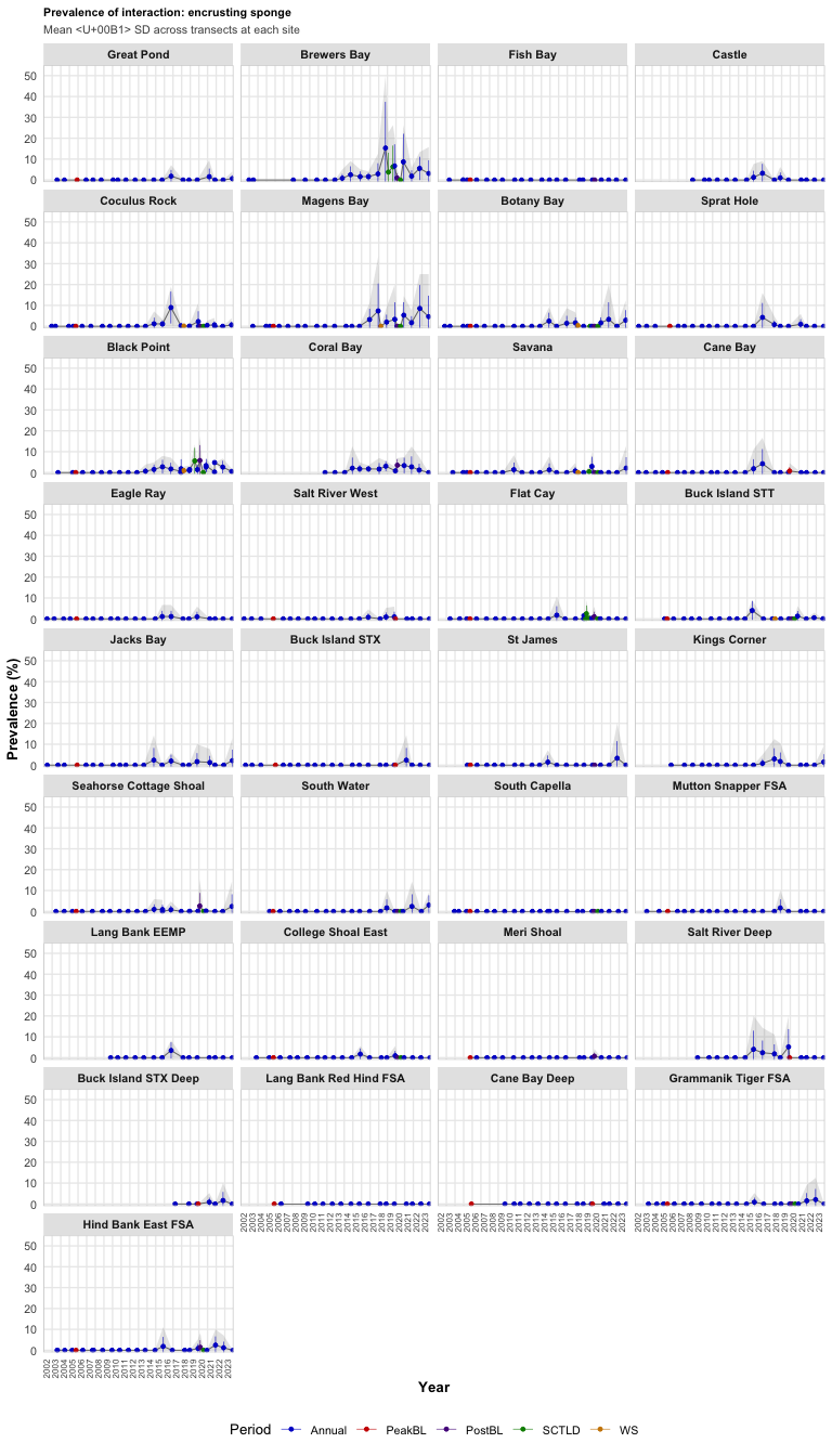
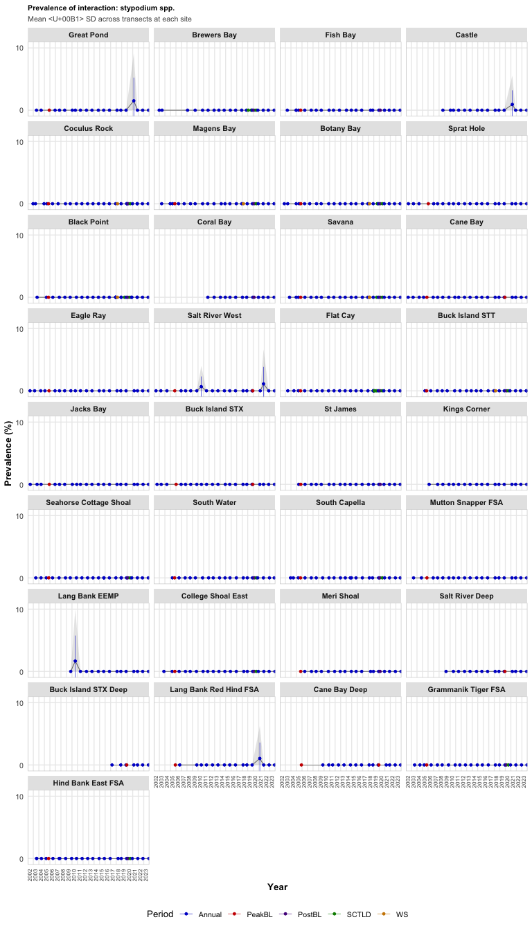
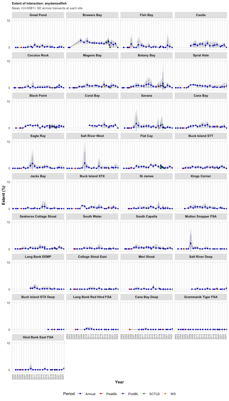
process_plot_healthdata This function creates a visual representation of coral interaction data trends over time for multiple sites.

  • Inputs: processed coral interaction data, column to plot, title (optional), y-label (optional), and facet column number
  • Process:
    1. Summarizes data by calculating mean values and standard deviations for each site and time point
    2. Creates a ggplot object with points for mean values and error bars for standard deviations
    3. Facets the plot by site for comparison
    4. Applies custom styling and labeling
  • Output: A ggplot object showing the trend of the specified coral interaction metric across sites and time
Show code
process_plot_healthdata <- function(data, column_to_plot, title = NULL, y_label = NULL, facet_ncol = 4, start_year, end_year) {
  # Ensure the column exists
  if (!column_to_plot %in% names(data)) {
    stop(paste("Column", column_to_plot, "not found in the data."))
  }
  
  # Set default title and y-label if not provided
  if (is.null(title)) {
    title <- paste("Coral", column_to_plot, "Over Time")
  }
  if (is.null(y_label)) {
    y_label <- paste(column_to_plot, "(%)")
  }
  
  # Convert start_yearand end_year to proper dates
  start_year<- as.Date(paste0(start_year, "-01-01"))
  end_year <- as.Date(paste0(end_year, "-12-31"))
  
  # Ensure 'date' is of Date type
  data <- data %>%
    mutate(date = as.Date(date))
  
  # Summarize the data
  summary_data <- data %>%
    group_by(site, date, period) %>%
    summarise(
      mean_value = mean(!!sym(column_to_plot), na.rm = TRUE),
      sd_value = sd(!!sym(column_to_plot), na.rm = TRUE),
      se_value = sd_value / sqrt(n()),
      lower_ci = mean_value - sd_value,
      # lower_ci = mean_value - sd_value,
      upper_ci = mean_value + sd_value,
      min_value = min(!!sym(column_to_plot), na.rm = TRUE),
      max_value = max(!!sym(column_to_plot), na.rm = TRUE),
      # upper_ci = mean_value + sd_value,
      .groups = "drop"
    ) %>%
    # Join with sitedat to get depth
    left_join(sitedat %>% dplyr::select(site, depth), by = "site") %>%
    # Reorder site from shallow to deep depths
    mutate(site = factor(site, levels = unique(site[order(depth)]))) %>%
    arrange(site, date)
  
  # Handle missing period values
  summary_data <- summary_data %>%
    mutate(period = ifelse(is.na(period), "No Data", period))
  
  # y limits 
  # ylim_min <- -max(summary_data %>% na.omit() %>% mutate(mmax = upper_ci) %>% pull(mmax))/10
  # ylim_max <- max(summary_data %>% na.omit() %>%  mutate(mmax = upper_ci) %>% pull(mmax))*1.1
  # 
  # ylim_min <- min(summary_data %>% na.omit() %>% mutate(mmin = min(lower_ci, min_value) %>% pull(mmin))*1.1)
  # ylim_max <- max(summary_data %>% na.omit() %>% mutate(mmax = max(upper_ci, max_value) %>% pull(mmax))*1.1)
  #                  
  ylim_min <- ifelse(is.na(min(
    c(summary_data$lower_ci, summary_data$min_value), na.rm = TRUE) * 1.1), -1, 
    min(c(summary_data$lower_ci, summary_data$min_value), na.rm = TRUE) * 1.1)
  
  ylim_min <- ifelse(ylim_min < -1, -1, ylim_min) # ensure minimum is not less than -1
  
  ylim_max <- ifelse(is.na(max(
    c(summary_data$upper_ci, summary_data$max_value), na.rm = TRUE) * 1.1), 10, 
    max(c(summary_data$upper_ci, summary_data$max_value), na.rm = TRUE) * 1.1)

  ylim_max <- ifelse(ylim_max > 100, 100, ylim_max) # ensure maximum is not greater than 10
  
  # example summary_data
  # summary_data <- data.frame(
  #   site = c("Site1", "Site1", "Site2", "Site2"),
  #   date = as.Date(c("2020-01-01", "2021-01-01", "2020-01-01", "2021-01-01")),
  #   period = c("Period1", "Period1", "Period2", "Period2"),
  #   mean_value = c(50, 60, 70, 80),
  #   sd_value = c(5, 6, 7, 8),
  #   se_value = c(2.5, 3, 3.5, 4),
  #   lower_ci = c(47.5, 54, 66.5, 76),
  #   upper_ci = c(52.5, 66, 73.5, 84)
  # )
  
  # if (is.infinite(ylim_max)) {
  #   ylim_min = -1 
  #   ylim_max = 10
  # }
  
  print(ylim_min)
  print(ylim_max)
  
  # Define custom colors (ensure it covers all periods)
  periods <- unique(summary_data$period)
  custom_colors <- c("blue3", "red3", "green4", "purple4", "orange3", "brown4", "pink3", "gray50")
  if (length(custom_colors) < length(periods)) {
    # Generate additional colors if needed
    custom_colors <- scales::hue_pal()(length(periods))
  }
  names(custom_colors) <- periods
  
  # Create the plot
  ggplot(summary_data, aes(x = date, y = mean_value, group=site)) +
    geom_ribbon(aes(ymin = min_value, ymax = max_value), fill = "gray50", alpha = 0.2) +
    geom_line(color="black",linewidth=0.2)+
    geom_point(size = 1, aes(color = period)) +
    geom_errorbar(aes(ymin = lower_ci, ymax = upper_ci, color = period), linewidth = 0.2) +
    facet_wrap(~site, ncol = facet_ncol) +
    scale_x_date(
      limits = c(start_year, end_year),
      date_breaks = "1 year",  # Adjust as needed
      date_labels = "%Y",
      expand = c(0, 0)
    ) +
    scale_y_continuous(
      expand = c(0, 0),
      breaks = if (ylim_max > 10) seq(0, 100, 10) else seq(0, 10, 2)) +
    # coord_cartesian(ylim = c(0, 100)) +  # Adjust y-limits to fit the data
    coord_cartesian(ylim = c(ylim_min,ylim_max)) + 

    # coord_cartesian(ylim = c(-0.5*max(summary_data %>% mutate(mmax = mean_value+upper_ci) %>% pull(mmax)), ceiling(max(summary_data %>% mutate(mmax = mean_value+upper_ci) %>% pull(mmax))))) + 
    # coord_cartesian(ylim = c(0-(0.1*ceiling(max(summary_data %>% mutate(mmax = mean_value+upper_ci) %>% pull(mmax)))), ceiling(max(summary_data %>% mutate(mmax = mean_value+upper_ci) %>% pull(mmax))))) + 

    scale_color_manual(values = custom_colors,guide = guide_legend(nrow = 1)) +
    labs(
      title = title,
      subtitle = "Mean ± SD across transects at each site",
      x = "Year",
      y = y_label,
      color = "Period"  # Update legend title
    ) +
    theme_minimal(base_size = 10) +
    theme(
      legend.position = "bottom",
      strip.background = element_rect(fill = "gray90", color = NA),
      strip.text = element_text(size=8, face = "bold"),
      panel.grid.minor = element_blank(),
      panel.border = element_rect(color = "gray80", fill = NA),
      plot.title = element_text(face = "bold", size = 8),
      plot.subtitle = element_text(size = 8, color = "gray30"),
      axis.title = element_text(face = "bold"),
      axis.text.x = element_text(size=6, angle = 90, hjust = 1)
    )
}

apply plotting functions

Show code
# Create separate lists to store faceted and overlaid plots
condition_plots_faceted <- list()
# condition_plots_overlaid <- list()

process_coltomeaning <- function(col2){
  if(col2 %in% gsub(" ","",tolower(input_benthiccodes$Meaning))){
      ind <- which(col2 == gsub(" ","",tolower(input_benthiccodes$Meaning)))
      input_benthiccodes$Meaning[ind[1]]
  } else {
    col2
  }
}

# Loop through each interaction category
for (category in condition_categories) {
  # Plot prevalence
  prevalence_data <- condition_list[[category]]$prevalence_summary
  prevalence_columns <- names(prevalence_data)[grep("^prev_", names(prevalence_data))]
  
  for (col in prevalence_columns) {
    plot_title <- paste("Prevalence of interaction:", 
                       tolower(process_coltomeaning(gsub("^prev_", "", col))))
    
    # Create faceted plot
    condition_plots_faceted[[paste(category, col)]] <- process_plot_healthdata(
      prevalence_data,
      col,
      plot_title,
      "Prevalence (%)",
      start_year = start_year_c,
      end_year = end_year_c
    )
    
  }
  
  # Plot extent
  extent_data <- condition_list[[category]]$extent_summary
  extent_columns <- names(extent_data)[grep("^ext_", names(extent_data))]
  
  for (col in extent_columns) {
    plot_title <- paste("Extent of interaction:", 
                       tolower(process_coltomeaning(gsub("^ext_", "", col))))
    
    # Create faceted plot
    condition_plots_faceted[[paste(category, col)]] <- process_plot_healthdata(
      extent_data, 
      col, 
      plot_title, 
      "Extent (%)", 
      start_year = start_year_c,
      end_year = end_year_c
    )
    
  }
}
[1] -1
[1] 18.33333
[1] -1
[1] 22
[1] -1
[1] 18.33333
[1] -1
[1] 9.166667
[1] -1
[1] 24.44444
[1] -1
[1] 44
[1] -1
[1] 10
[1] -1
[1] 15.71429
[1] -1
[1] 7.857143
[1] -1
[1] 13.75
[1] -1
[1] 22
[1] -1
[1] 13.75
[1] -1
[1] 14.34783
[1] -1
[1] 55
[1] -1
[1] 10
[1] -1
[1] 22
[1] 0
[1] 0
[1] -1
[1] 55
[1] 55
[1] 100
[1] -1
[1] 11
[1] -1
[1] 22
[1] -1
[1] 11
[1] -1
[1] 22
[1] -1
[1] 11
[1] -1
[1] 11
[1] -1
[1] 8.8
[1] -1
[1] 11
[1] -0.7972194
[1] 3.3
[1] -1
[1] 5.5
[1] -1
[1] 11
[1] -1
[1] 22
[1] -1
[1] 16.5
[1] -1
[1] 39.6
[1] -1
[1] 17.6
[1] -0.5438699
[1] 2.2
[1] 0
[1] 0
[1] -1
[1] 39.6
[1] -1
[1] 100
[1] -1
[1] 100
[1] -1
[1] 69.47368
[1] -1
[1] 97.30769
[1] -1
[1] 100
[1] -1
[1] 100
[1] 0
[1] 100
[1] -1
[1] 93.5
[1] -1
[1] 100
[1] -1
[1] 100
[1] -1
[1] 100
[1] -1
[1] 100
[1] -1
[1] 100
[1] -1
[1] 36.66667
[1] -1
[1] 70
[1] -1
[1] 36.66667
[1] -1
[1] 36.66667
[1] -1
[1] 15.71429
[1] -1
[1] 29.33333
[1] -1
[1] 70
[1] 40
[1] 100
[1] -1
[1] 77
[1] -1
[1] 44
[1] -1
[1] 38.5
[1] -1
[1] 22
[1] -1
[1] 11
[1] -1
[1] 44
[1] -1
[1] 77
[1] -1
[1] 100
[1] -1
[1] 100
[1] -1
[1] 45.29412
[1] -1
[1] 93.07692
[1] -1
[1] 77.64706
[1] -1
[1] 100
[1] -1
[1] 55
[1] -1
[1] 62.85714
[1] -1
[1] 91.66667
[1] -1
[1] 39.28571
[1] -1
[1] 73.33333
[1] -1
[1] 14.34783
[1] -1
[1] 22
[1] -1
[1] 22
[1] -1
[1] 31.42857
[1] -1
[1] 8.461538
[1] -1
[1] 8.461538
[1] -1
[1] 9.166667
[1] -1
[1] 14.66667
[1] -1
[1] 11
[1] -1
[1] 55
[1] -1
[1] 18.33333
[1] -1
[1] 10
[1] -1
[1] 71.17647
[1] -0.4049791
[1] 8.490449
[1] 0
[1] 0
[1] -1
[1] 8.461538
[1] -1
[1] 100
[1] -1
[1] 100
[1] -1
[1] 47.66667
[1] -1
[1] 55
[1] -1
[1] 88
[1] -1
[1] 55
[1] -1
[1] 55
[1] -1
[1] 27.5
[1] -1
[1] 93.5
[1] -1
[1] 49.5
[1] -1
[1] 23.83333
[1] -1
[1] 44
[1] -1
[1] 9.9
[1] -1
[1] 33
[1] -1
[1] 22
[1] -1
[1] 7.7
[1] -0.5314796
[1] 2.2
[1] -1
[1] 66
[1] -1
[1] 5.5
[1] -1
[1] 5.5
[1] -1
[1] 22
[1] -0.7972194
[1] 3.3
[1] -1
[1] 16.5
[1] -1
[1] 11
[1] -1
[1] 15.4
[1] -1
[1] 8.8
[1] 0
[1] 0
[1] -0.7972194
[1] 3.3
[1] -1
[1] 55
[1] -1
[1] 100
[1] -1
[1] 36.66667
[1] -1
[1] 27.5
[1] -1
[1] 100
[1] -1
[1] 4.583333
[1] -1
[1] 36.66667
[1] -1
[1] 8.461538
[1] -1
[1] 31.42857
[1] -1
[1] 15
[1] -1
[1] 22
[1] -1
[1] 27.5
[1] -1
[1] 100
[1] -1
[1] 29.33333
[1] -1
[1] 12.22222
[1] -1
[1] 22
[1] -1
[1] 18.33333
[1] -1
[1] 12.22222
[1] -1
[1] 7.333333
[1] -1
[1] 8.461538
[1] -1
[1] 11
[1] -1
[1] 10
[1] -1
[1] 6.875
[1] -1
[1] 5.789474
[1] -1
[1] 10
[1] -1
[1] 15.71429
[1] -1
[1] 10
[1] -1
[1] 5
[1] 0
[1] 0
[1] -0.9490707
[1] 3.928571
[1] -1
[1] 100
[1] -1
[1] 100
[1] -1
[1] 100
[1] -1
[1] 100
[1] -1
[1] 100
[1] -1
[1] 5.5
[1] -1
[1] 16.5
[1] -0.2657398
[1] 1.1
[1] -1
[1] 88
[1] -1
[1] 22
[1] -1
[1] 22
[1] -1
[1] 22
[1] -1
[1] 33
[1] -1
[1] 13.27817
[1] -0.7972194
[1] 3.983452
[1] -0.5314796
[1] 2.2
[1] -1
[1] 13.27817
[1] -1
[1] 16.5
[1] -1
[1] 5.5
[1] -0.7972194
[1] 3.3
[1] -1
[1] 11
[1] -1
[1] 5.5
[1] -0.5314796
[1] 2.2
[1] -1
[1] 11
[1] -1
[1] 11
[1] -1
[1] 22
[1] -1
[1] 7.7
[1] -1
[1] 11
[1] 0
[1] 0
[1] -0.2657398
[1] 1.1
[1] -1
[1] 100
[1] -1
[1] 100
[1] -1
[1] 100
[1] -1
[1] 36.66667
[1] -1
[1] 4.230769
[1] -1
[1] 32.35294
[1] -1
[1] 36.66667
[1] -1
[1] 12.22222
[1] -1
[1] 48.88889
[1] -1
[1] 68.75
[1] -1
[1] 20.625
[1] -1
[1] 11.57895
[1] -1
[1] 17.1875
[1] -1
[1] 7.333333
[1] -1
[1] 6.470588
[1] -1
[1] 5.238095
[1] -1
[1] 5.789474
[1] -1
[1] 16.92308
[1] -1
[1] 100
[1] 0
[1] 100
[1] -1
[1] 93.5
[1] -1
[1] 45.65
[1] -1
[1] 6.6
[1] -1
[1] 5.5
[1] -1
[1] 44
[1] -1
[1] 16.5
[1] -1
[1] 5.5
[1] -1
[1] 22
[1] -1
[1] 14.3
[1] -1
[1] 8.8
[1] -1
[1] 8.36
[1] -1
[1] 5.5
[1] -1
[1] 38.5
[1] -1
[1] 5.5
[1] -1
[1] 11
[1] -1
[1] 13.2
[1] -1
[1] 93.5
[1] -1
[1] 100
[1] -1
[1] 40
[1] -1
[1] 25
[1] -1
[1] 78.57143
[1] -1
[1] 55
[1] -1
[1] 24.44444
[1] -1
[1] 47.14286
[1] -1
[1] 24.44444
[1] -1
[1] 13.75
[1] -1
[1] 15.71429
[1] -1
[1] 80
[1] 30
[1] 100
[1] -1
[1] 44
[1] -0.2657398
[1] 1.371935
[1] -1
[1] 55
[1] -1
[1] 30.25
[1] -1
[1] 27.5
[1] -1
[1] 49.5
[1] -1
[1] 100
[1] -1
[1] 33
[1] -1
[1] 22
[1] -1
[1] 100
[1] -1
[1] 100
[1] -1
[1] 55
[1] -1
[1] 22
[1] -1
[1] 66
[1] -1
[1] 16.5
[1] -1
[1] 27.5
[1] -1
[1] 66
[1] 44
[1] 100
[1] -1
[1] 23.1
[1] -1
[1] 6.6
[1] -1
[1] 20.9
[1] -1
[1] 7.7
[1] -0.5454095
[1] 3.3
[1] -1
[1] 20.9
[1] -1
[1] 100
[1] -1
[1] 59.23077
[1] -1
[1] 36.66667
[1] -1
[1] 12.22222
[1] -1
[1] 6.875
[1] -1
[1] 25.88235
[1] -1
[1] 11
[1] -1
[1] 15.71429
[1] -1
[1] 13.75
[1] -1
[1] 67.69231
[1] 42.30769
[1] 100
[1] -1
[1] 35.2
[1] -1
[1] 24.2
[1] -0.5314796
[1] 2.2
[1] -0.5438699
[1] 2.2
[1] -1
[1] 9.35
[1] -1
[1] 16.5
[1] -0.7208816
[1] 3.85
[1] -1
[1] 17.6
[1] -1
[1] 35.2
[1] -1
[1] 100
[1] -1
[1] 100
[1] -1
[1] 40
[1] -1
[1] 41.25
[1] -1
[1] 47.14286
[1] -1
[1] 30
[1] -1
[1] 13.75
[1] -1
[1] 55
[1] -1
[1] 15.71429
[1] -1
[1] 100
[1] 0
[1] 100
[1] -1
[1] 4.4
[1] -1
[1] 11
[1] -0.5314796
[1] 2.2
[1] -1
[1] 5.5
[1] -0.5314796
[1] 2.2
[1] -0.5314796
[1] 2.2
[1] -1
[1] 4.4
[1] -0.2013709
[1] 1.1
[1] -1
[1] 11
[1] -1
[1] 100
Show code
# Display the first few plots of each type as an example
cat("\nFaceted Plots:\n")

Faceted Plots:
Show code
  print(sample(condition_plots_faceted, 3))
$`Damselfish ext_anydamselfish`


$`Sponge prev_encrustingsponge`


$`Macroalgae prev_stypodiumspp.`

save plots

Downloads

loop thru download links :

Coral condition: Coral

Coral condition: Cyanobacteria

Coral condition: Gorgonian

Coral condition: Macroalgae

Coral condition: Other

Coral condition: Predation

Coral condition: Sponge

Coral condition: Worm

Coral condition: Corallivore

Coral condition: Damselfish