Show code
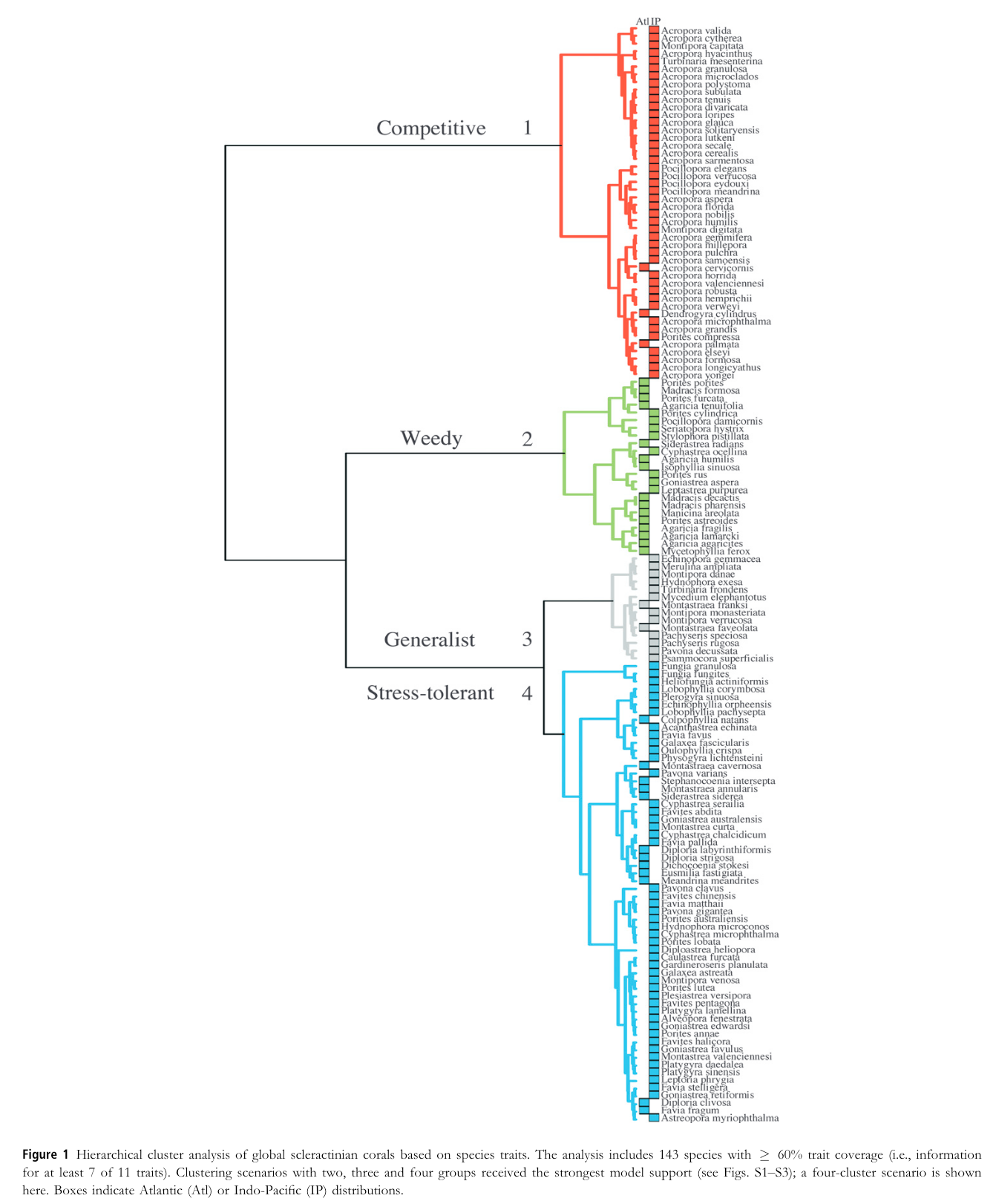
load("benthicCoverXrefBenthicCodes.RData")This page assigns each surveyed coral taxon to one of four life-history trait groups from Darling et al. (2012) (competitive, weedy, generalist, stress-tolerant), then sums percent cover within each group and averages it by site and year across the three monitoring programs (TCRMP, VINPS, CSUN). The classification follows Darling et al. (2012) with one update from more recent literature: Millepora joins the competitive life-history category, because it shares ecological traits with Acropora, the other emblematic competitive coral taxon (Cramer et al. 2021). The page produces the site-faceted trait-group cover time series in Figure 1 and the downloadable long-format table s2pt6_benthicCoverCoralTraitGroup, which the resilience and publication pages read downstream.
This page reads the reformatted, cross-referenced benthic-cover workspace written upstream by 01_reformat_data.qmd and 02_xref_benthic_codes.qmd, which combine the three monitoring programs: TCRMP, VINPS, and CSUN. The workspace holds the per-program reformatted benthic-cover data and the shared benthic-code cross-reference that carries the trait classifications, all held to the site embargo (data through 2023). This page’s own derived output is available in the Downloads section below.
What happens here: the page loads the reformatted, cross-referenced benthic-cover workspace from parts 1 and 2, then sets the grouping variable that drives every step below.
load("benthicCoverXrefBenthicCodes.RData")groupingvar names the column of benthicCodes used to group taxa on this page (coralTraits), and section sets the output-file prefix (s2pt6).
# subfoldername <- "benthicCoverGrouped"
groupingvar <- "coralTraits"
section <- "s2pt6" # for namingbenthicDat into subgroupings of interestThis step filters benthicCodes down to the coral taxa that carry a trait classification. It keeps coral rows, drops rows with no assigned trait, and unsets the CSUN Millepora trait so it is handled consistently with the other programs.
getBenthicDatColInds()this is one of two functions that connect benthicDat to benthicCodes for all three programs.
getBenthicDatColInds() makes _columnInds that stores column indices of benthic codes corresponding to each item of coralTraits
arguments:
benthicDat is benthic dataset of interest
codecolumn is the name of the column of benthic code containing the code for benthicdat
groupingcolumn is the name of the column of benthic codes where the grouping variable of interest is stored.
getBenthicDatColInds <-
  function(benthicDat, codecolumn, groupingcolumn) {
    codecolind <-
      which(colnames(benthicCodes) == codecolumn)
    groupingcolind <-
      which(colnames(benthicCodes) == groupingcolumn)
    genusdf <-
      data.frame(group =
                   unique(benthicCodes[, groupingcolind]),
                 colinds =
                   rep(0, length(unique(benthicCodes[, groupingcolind]))))
    for (i in 1:nrow(genusdf)) {
      codei <-
        benthicCodes[which(benthicCodes[, groupingcolind] == genusdf$group[i]), ]
      genusdf$colinds[i] <-
        list(which(colnames(benthicDat) %in% codei[, codecolind]))
    }
    # UAGA-guard: warn on benthicDat data columns whose code is absent from benthicCodes and is
    # therefore silently dropped (the footgun that lost VINPS Agaricia agaricites, code UAGA).
    .known <- benthicCodes[[codecolind]]; .known <- .known[nchar(.known) > 0]
    .meta_cols <- c("program","date","site","period","replicate","replicatetype","nopts",
                    "Year","Date","SiteFullName","year","month","percentCover_allCoral",
                    "PC","Check","Notes","Transect")
    .dropped <- setdiff(colnames(benthicDat), c(.known, .meta_cols))
    if (length(.dropped) > 0)
      warning("getBenthicDatColInds(", codecolumn, "): ", length(.dropped),
              " data column(s) have codes absent from benthicCodes and are DROPPED: ",
              paste(.dropped, collapse = ", "), " -- add them to benthicCodes if they are taxa.")
    return(genusdf)
  }
The page applies getBenthicDatColInds() to each program’s benthic data, mapping every trait group to the data columns that belong to it.
tcrmp_columnInds <-
  getBenthicDatColInds(tcrmp_benthicDat, "tcrmp_Code", "tcrmp_trait")
vinps_columnInds <-
  getBenthicDatColInds(vinps_benthicDat, "vinps_TaxonCode", "tcrmp_trait")
csunrandom_columnInds <-
getBenthicDatColInds(csun_random_benthicDat, "csun_random_code", "tcrmp_trait")getBenthicDatColInds() resolves the trait groups competitive, generalist, stresstolerant, weedy for TCRMP. The UAGA guard inside the function warns if any data column carries a taxon code that is absent from benthicCodes (the footgun that once dropped VINPS Agaricia agaricites); watch the render log for that warning when new data or codes arrive.
makeGroupedBenthicDat()this is the second function that connects benthicDat to benthicCodes for all three programs.
makeGroupedBenthicDat() extracts the column indices (colinds) from each row of *_columnInds.
If only one index in colinds , assigns the corresponding column from benthicdat to the i-th column of a data frame _groupedBenthicDat.
if more than one index in colinds, stores row sum of benthicDat[,colinds] in the i-th column of _groupedBenthicDat.
arguments:
benthicDat is benthic dataset of interest
columnInds is the output of getBenthicDatColInds() above that contains column indices of benthic codes for each benthic subgroup of interest
makeGroupedBenthicDat <- function(benthicDat, columnInds) {
  groupeddat <- data.frame(matrix(nrow = nrow(benthicDat),
                                  ncol = nrow(columnInds)))
  colnames(groupeddat) <- columnInds$group
  benthicDat <- benthicDat %>% dplyr::mutate(dplyr::across(dplyr::where(is.numeric), ~replace(.x, is.na(.x), 0)))
  for (i in 1:nrow(columnInds)) {
    geni <- columnInds[i,]
    datcoli <- unlist(geni$colinds)
    if (length(datcoli) == 1) {
      groupeddat[, i] <- benthicDat[, datcoli]
    } else {
      groupeddat[, i] <- rowSums(benthicDat[, datcoli])
    }
  }
  groupeddat <- cbind(benthicDat[, 1:6], groupeddat)
  return(groupeddat)
}
The page applies makeGroupedBenthicDat() to each program, producing one trait-group cover value per survey record.
tcrmp_groupedBenthicDat <-
  makeGroupedBenthicDat(tcrmp_benthicDat, tcrmp_columnInds)
vinps_groupedBenthicDat <-
  makeGroupedBenthicDat(vinps_benthicDat, vinps_columnInds)
csun_groupedBenthicDat <-
  makeGroupedBenthicDat(csun_random_benthicDat, csunrandom_columnInds)
The grouped TCRMP table now holds 4,412 survey records with the trait-group cover columns competitive, generalist, stresstolerant, weedy alongside the six survey-identifier columns.
benthicDat from three programsnow have three _groupedBenthicDat, need to merge them, start by comparing the column names, because some are missing from csun.
make sure each _groupedBenthicDat has the same column names
for (col in missing_columns_tcrmp) {
  tcrmp_groupedBenthicDat[[col]] <- NA
}
for (col in missing_columns_vinps) {
  vinps_groupedBenthicDat[[col]] <- NA
}
for (col in missing_columns_csung) {
  csun_groupedBenthicDat[[col]] <- NA
}tcrmp_groupedBenthicDat <- tcrmp_groupedBenthicDat[, all_columns]
vinps_groupedBenthicDat <- vinps_groupedBenthicDat[, all_columns]
csun_groupedBenthicDat <- csun_groupedBenthicDat[, all_columns]groupedBenthicDat.groupedBenthicDat <-
rbind(tcrmp_groupedBenthicDat,
vinps_groupedBenthicDat,
csun_groupedBenthicDat)groupedBenthicDat into long format.For TCRMP and VINPS, this page averages transect-level percent cover to an annual site value and carries the standard error across transects. CSUN has no transect replicate at the site level, so its cover is summed as cumulative cover per site rather than transect-averaged, and its points carry no error term.
The three programs do not share a sampling structure. TCRMP and VINPS survey replicate transects per site, so their site-year values are transect means with a standard error. CSUN has no transect replicate, so its cover is cumulative per site and shows no error bar. The programs also span different windows (TCRMP and VINPS begin in the 1990s, CSUN records reach back to 1987). Read across-program comparisons in Figure 1 with these differences in mind. The error bars are within-program only, never pooled across programs.
The first summary collapses trait-group cover to total coral cover per transect, then averages transects to a site-year mean with a standard error. These are the black total-cover points in Figure 1.
totaldatCovSum <- groupedBenthicDat |>
  dplyr::group_by(year, date, program, site, period, replicate) |>
  dplyr::summarise(perccover = sum(perccover))

totaldatCovSum <- totaldatCovSum |>
  dplyr::group_by(year, date, program, site) |>
  dplyr::summarise(
    meancov = mean(perccover),
    sdcov = sd(perccover),
    secov = sd(perccover) / (sqrt(length(perccover))),
    n = length(perccover)
  )

totaldatCovSum <- totaldatCovSum %>% dplyr::mutate(dplyr::across(dplyr::where(is.numeric), ~replace(.x, is.na(.x), 0)))The second summary keeps the trait groups separate, giving the stacked areas in Figure 1: mean cover per trait group per site and year.
groupedBenthicDatCovSum <- groupedBenthicDat |>
  dplyr::group_by(year, date, program, site, period, coralTraits) |>
  dplyr::summarise(
    meancov = mean(perccover),
    sdcov = sd(perccover),
    secov = sd(perccover) / (sqrt(length(perccover))),
    n = length(perccover)
  )
groupedBenthicDatCovSum <- groupedBenthicDatCovSum %>% dplyr::mutate(dplyr::across(dplyr::where(is.numeric), ~replace(.x, is.na(.x), 0)))Figure 1 shows how coral cover splits among the four life-history trait groups at each site through time. Reading a site’s stacked area shows whether its coral is dominated by competitive, weedy, generalist, or stress-tolerant taxa, and whether that mix shifts after disturbance. Sites are ordered shallow to deep, and the dashed line marks the 2005 bleaching event.
#add site info so can plot according to increasing depth
groupedBenthicDatCovSum <-
  merge(groupedBenthicDatCovSum, sitedat, by = "site")
groupedBenthicDatCovSum <-
  groupedBenthicDatCovSum[order(groupedBenthicDatCovSum$depth), ]
groupedBenthicDatCovSum$site <- factor(groupedBenthicDatCovSum$site,
                                       levels = unique(groupedBenthicDatCovSum$site))

#add site info so can plot according to increasing depth
totaldatCovSum <-
  merge(totaldatCovSum, sitedat, by = "site")
totaldatCovSum <-
  totaldatCovSum[order(totaldatCovSum$depth), ]
totaldatCovSum$site <- factor(totaldatCovSum$site,
                              levels = unique(totaldatCovSum$site))

create_stacked_area_plot <- function(data_stacked, data_total,
                                                x_var = "year", y_var = "meancov",
                                                fill_var = "coralTraits", facet_var = "site",
                                                error_var = "secov",
                                                min_year = NULL, max_year = NULL,
                                                highlight_year = NULL,
                                                max_facets_per_page = 35) {

  # Determine x-axis limits if not provided
  if (is.null(min_year))
    min_year <- floor(min(data_stacked[[x_var]]))
  if (is.null(max_year))
    max_year <- ceiling(max(data_stacked[[x_var]]))

  # Calculate optimal number of rows and columns
  n_facets <- length(unique(data_stacked[[facet_var]]))
  n_facets <- min(n_facets, max_facets_per_page)  # Limit to max_facets_per_page
  n_col <- ceiling(sqrt(n_facets))
  n_row <- ceiling(n_facets / n_col)

  # Create base plot
  p <- ggplot() +
    geom_area(data = data_stacked,
              aes(x = .data[[x_var]], y = .data[[y_var]], fill = .data[[fill_var]]),
              position = 'stack') +
    geom_point(
      data = data_total,
      aes(x = .data[[x_var]], y = .data[[y_var]]),
      color = "black",
      size = 0.5
    ) +
    geom_linerange(
      data = data_total,
      aes(
        x = .data[[x_var]],
        ymin = .data[[y_var]] - .data[[error_var]],
        ymax = .data[[y_var]] + .data[[error_var]]
      ),
      color = "black",
      linewidth = 0.5
    ) +
    facet_wrap(vars(.data[[facet_var]]), nrow = n_row, ncol = n_col, scales = "free_x") +
    labs(y = "Percent cover", x = toupper(x_var)) +
    scale_y_continuous(expand = c(0, 0)) +
    scale_x_continuous(
      expand = expansion(mult = 0.04),
      breaks = seq(min_year, max_year, by = 1),
      labels = function(x)
        ifelse(x %% 5 == 0, paste0("'", substr(x, 3, 4)), "")
    ) +
    theme_bw() +
    theme(
      strip.text = element_text(size = 10),
      legend.position = "bottom",
      panel.grid = element_blank()
    )

  # Add highlight line if specified
  if (!is.null(highlight_year)) {
    p <- p + geom_vline(
      xintercept = highlight_year,
      color = "gray50",
      alpha = 0.5,
      linetype = "dashed"
    )
  }

  return(p)
}

# Usage:
stack <- create_stacked_area_plot(
  data_stacked = groupedBenthicDatCovSum,
  data_total = totaldatCovSum,
  min_year = minyear,
  max_year = maxyear,
  highlight_year = 2005,
  fill_var = "coralTraits",
  max_facets_per_page = length(unique(groupedBenthicDatCovSum$site))
)

# Display the plot
print(stack)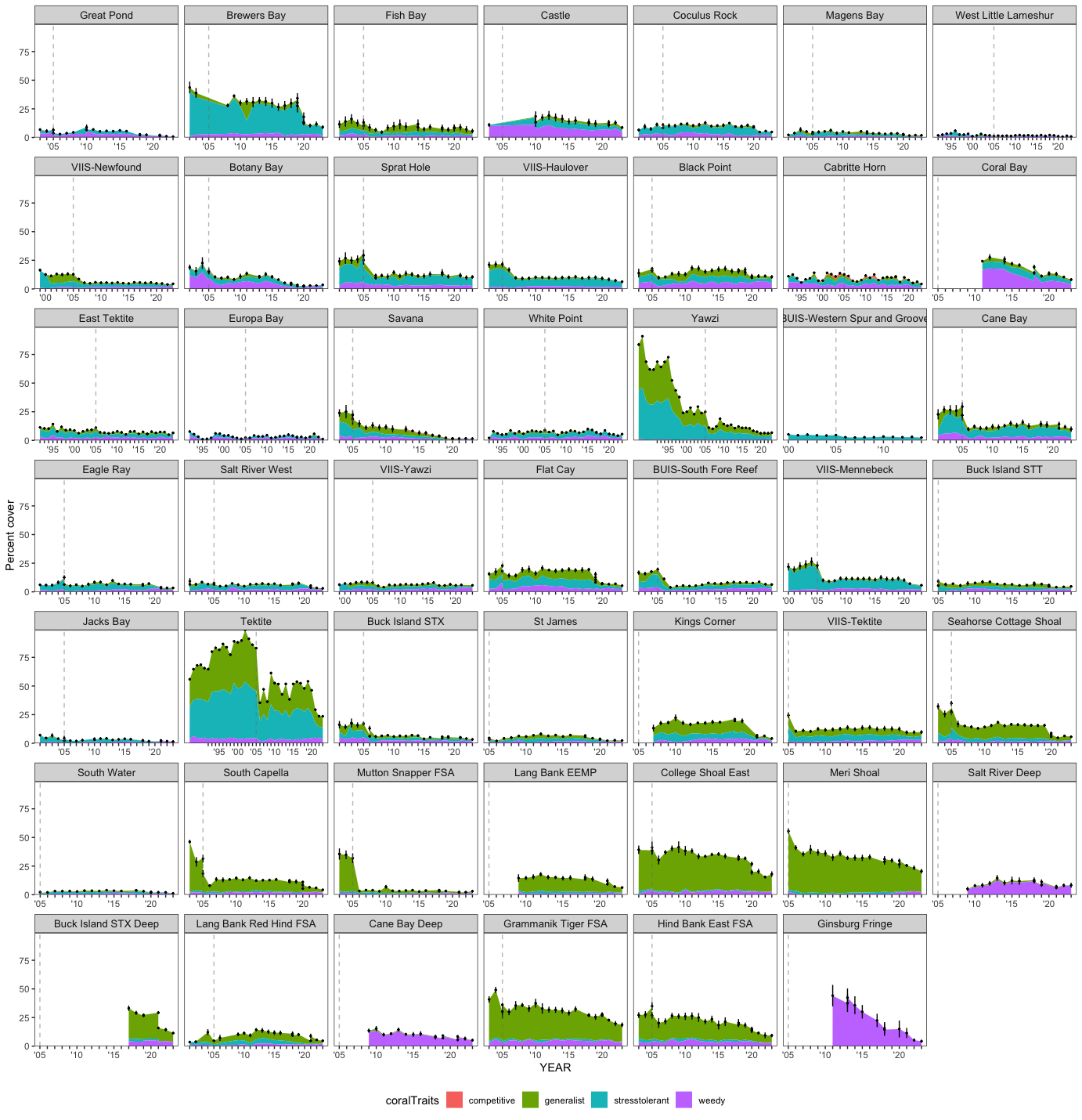
Trait-group composition tracks each site’s disturbance history. Where a site’s stacked area thins after 2005 and refills with weedy or stress-tolerant cover rather than competitive cover, the coral community has shifted toward a lower-relief, disturbance-associated state. Figure 1 makes that shift visible site by site and program by program.
This page writes the coral trait-group cover product s2pt6_benthicCoverCoralTraitGroup (one row per site, year, and trait group) plus its metadata. The download links below are generated from the same object the page computes, so the file and its provenance travel together.
Figure 1 faces 49 sites in one static frame. A Shiny explorer would let a reader pick sites, programs, and a year window and read a small, legible facet set instead of the full wall.
s2pt6_benthicCoverCoralTraitGroup (this page’s output) joined to site depth and program.version 1.0.0 • in-review • data ≤ 2023