4.6 Currents
4.6 Currents
On this page
This page summarizes modeled seawater currents at the VIRRS sites for the year 2019. We read hourly zonal (east-west) and meridional (north-south) current components from ROMS model outputs, convert each hourly pair into a current speed and direction, and reduce the full year into per-site descriptors: mean and 95th-percentile speed with their associated directions, the top-decile mean speed, and the daily rate of speed pulses and directional-change pulses. The page produces a site map showing mean current speed and direction (Figure 3), and writes one per-site summary table with its metadata. This is a single-year snapshot from a model, not a monitoring time series, so it holds no program-specific trend and carries no error bars.
Data sources
This page reads ROMS current model outputs for 2019 (hourly zonal and meridional components at every VIRRS site), described on the currents entry of the Data Sources page. Site coordinates come from the site master. The derived per-site current summary produced here is available in the Downloads section below.
Import current data and set the record length
We read two hourly current fields for every site:
-
current_z= zonal (east-west) current -
current_m= meridional (north-south) current -
ndays= the number of days the current data span.
We drop incomplete rows and convert the number of hourly readings into a record length in days.
Show code
current_z <- current_z[complete.cases(current_z),]
current_m <- current_m[complete.cases(current_m),]

ndays <- nrow(current_z)/24

#convert ndays to min and max calendar date
start_date <- as_datetime("2019-01-01 00:00:00")
end_date <- as_datetime(start_date + ndays * 24 * 60 * 60)
The record spans 359.75 days (2019-01-01 to 2019-12-26 18:00:00) at 1-hour timesteps.
Function: speed and direction from zonal and meridional components
The current_calculations function takes a zonal (u) and a meridional (v) value and returns the current speed (magnitude, m/s) and direction (azimuth, degrees from north). It is adapted from rNOMADS::MagnitudeAzimuth.
Show code
current_calculations <- function(zonal.wind, meridional.wind) {
   #Given zonal (East-West) and meridional (North-South) wind speeds, calculate magnitude and azimuth.
   #INPUTS
   #    ZONAL.WIND - Wind East West, in meters per second, west negative
   #    MERIDIONAL.WIND - Wind North South, in meters per second, south negative
   #OUTPUTS
   #   MAGNITUDE - Wind magnitude, in meters per second
   #   AZIMUTH  - Wind azimuth, in degrees from north

   mag <- sqrt(zonal.wind^2 + meridional.wind^2)
   tmp.az <- (180/pi) * atan2(zonal.wind, meridional.wind)
   az <- tmp.az
   az[tmp.az < 0] <- 360 + tmp.az[tmp.az < 0]
   # return(data.frame(magnitude = mag, azimuth = az))
   return(data.frame(speed = mag, direction = az))
}
Per-site descriptive statistics
For each site, we convert every hourly zonal and meridional value into a speed and direction, then extract the mean, the 95th-percentile speed and its associated direction, and the top-decile mean (the average of the fastest 10% of speeds).
We initialize the currents_sum dataframe that collects one row per site.
Show code
currents_sum <- data.frame(
  program = character(0),
  site = character(0),
  lat = numeric(0),
  lon = numeric(0),
  quantile95Speed = numeric(0),
  quantile95SpeedDirection = numeric(0),
  meanSpeed = numeric(0),
  meanDirection = numeric(0),
  sdSpeed = numeric(0),
  sdDirection = numeric(0),
  meanu = numeric(0),
  meanv = numeric(0),
  quantile95u = numeric(0),
  quantile95v = numeric(0),
  top_decile_mean = numeric(0)
)
We iterate through each site, apply current_calculations to that site’s zonal and meridional values, then compute the mean, standard deviation, and 95th percentile of the resulting speed and direction values.
Show code
for (i in 1:ncol(current_m)) {
  data <- data.frame(u = current_z[, i],
                     v = current_m[, i])

  results <- data |>
    rowwise() |>
    do(current_calculations(.$u, .$v))

  # average speed: average All u and v components separately and "current_calculations" of resulting averages.
  data_mean <- current_calculations(mean(data$u), mean(data$v))
  data_sd <- current_calculations(sd(data$u), sd(data$v))

  # average directions: Add up all the north-south components.  Then separately, add up all the east/west components. The average direction is the arctan of the east/west components divided by the north south components. Dir = arctan(sum(Cew) / sum(Cns)) this ends up being same as data_mean$direction!
  # data_mean_direction <-
  #   atan(sum(data$u)/sum(data$v)) * (180 / pi)

  #calculate the 95%ile speed
  quantile_95_speed <- quantile(results$speed, probs = 0.95)
  quantile_95_speed_index <-
    which.min(abs(results$speed - as.numeric(quantile_95_speed)))

  # Calculate average of the top 10% speeds (aka top decile mean)
  top_10_percent <-
    results$speed[order(-results$speed)][1:floor(0.10 * length(results$speed))]
  average_top_10_percent <- mean(top_10_percent)

  # add to currents_sum
  indi <- which(gsub("-"," ",sitedat$site) == gsub("\\.", " ", colnames(current_m)[i]))

  currents_sum <- rbind(
    currents_sum,
    data.frame(
      program = sitedat$program[indi],
      site = sitedat$site[indi],
      lat = sitedat$lat[indi],
      lon = sitedat$lon[indi],
      quantile95Speed = quantile_95_speed,
      quantile95SpeedDirection = results$direction[quantile_95_speed_index],
      meanSpeed = data_mean$speed,
      meanDirection = data_mean$direction,
      sdSpeed = data_sd$speed,
      sdDirection = data_sd$direction,
      meanu = mean(data$u),
      meanv = mean(data$v),
      quantile95u = data$u[quantile_95_speed_index],
      quantile95v = data$v[quantile_95_speed_index],
      top_decile_mean = average_top_10_percent
    )
  )
}
Pulsed current events from hourly readings
Some reefs experience pulsed current events, short bursts where current speed jumps or the direction swings sharply. These pulses can arise from tidal changes, storm surges, or other oceanographic events. They influence planktonic food availability and larval dispersal, and can mark a system that is regularly perturbed. We count both speed pulses and directional-change pulses per site.
Speed pulses
We first convert current_m and current_z to numeric matrices.
Show code
current_m <-
  matrix(as.numeric(as.matrix(current_m)), ncol = ncol(current_m))
current_z <-
  matrix(as.numeric(as.matrix(current_z)), ncol = ncol(current_z))
We compute current speed for each site, then the hour-to-hour change in speed.
A speed pulse is an hourly increase larger than the 90th percentile of all speed changes, so we set that global threshold.
Show code
thold <- quantile(speed_difference, 0.90, na.rm = TRUE)We define a helper that returns, for one site, the hours whose speed change exceeds the threshold.
We apply it to every site to get the pulse events per site.
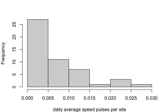
We count the pulses per site and divide by the record length to get an average number of speed pulses per day.
Show code
speedpulses <- lengths(pulses_speed)/ndays
speedpulses <- speedpulses / ndays
Figure 1 shows how the daily speed-pulse rate is distributed across sites.
Directional-change pulses
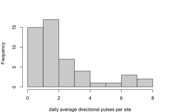
A rapid change in direction can influence nutrient distribution and sediment displacement. We treat an absolute change of 90 degrees or more between consecutive hours as a directional pulse.
We compute the direction at each hour, then the hour-to-hour change.
Because direction is circular, we wrap changes larger than 180 degrees back into the -180 to 180 range.
Show code
direction_diffs[direction_diffs > 180] <-
  direction_diffs[direction_diffs > 180] - 360

direction_diffs[direction_diffs < -180] <-
  direction_diffs[direction_diffs < -180] + 360
We flag the hours where the direction changed by more than 90 degrees.
We count them per site and divide by the record length for a daily rate.
Show code
dirpulses <- lengths(pulses_direction)
dirpulses <- dirpulses / ndays
Figure 2 shows how the daily directional-pulse rate is distributed across sites.
Show code
We add both pulse rates to currents_sum.
Show code
currents_sum$speedpulses <- speedpulses
currents_sum$dirpulses <- dirpulses
Current map
Figure 3 maps mean current speed and direction at each site. Arrow length encodes mean current speed and arrow orientation encodes mean current direction, drawn over the island coastlines.
Show code
background_map <-
  st_read(dsn = "../shapefiles/pvishrpl/", layer = "pvishrpl", quiet = TRUE)
lon_range <- range(sitedat$lon)
lat_range <- range(sitedat$lat)


p <- ggplot() +
  # Plot the background map
  geom_sf(data = background_map, fill = "grey50", color = "white") +
  # geom_point(
  #   data = currents_sum,
  #   aes(
  #     x = lon,
  #     y = lat,
  #     size = speedpulses,
  #     col = dirpulses
  #   ),
  #   alpha = 1
  # ) +
  scale_color_gradient(low = "darkblue", high = "magenta") +
  geom_segment(
    data = currents_sum,
    aes(
      x = lon,
      y = lat,
      xend = lon + meanu / 1,
      yend = lat + meanv / 1
    ),
    arrow = arrow(type = "closed", length = unit(0.05, "inches")),
    col = "black",
    size = 0.2
  ) +
  # geom_segment(
  #   data = currents_sum,
  #   aes(
  #     x = lon,
  #     y = lat,
  #     xend = lon + quantile95u / 3,
  #     yend = lat + quantile95v / 3
  #   ),
  #   arrow = arrow(type = "closed", length = unit(0.05, "inches")),
  #   color = "red",
  #   size = 0.2
  # ) +
  geom_point(data = currents_sum,
             aes(
               x = lon,
               y = lat,
               text = paste(
                 "site: ",
                 currents_sum$site,
                 "\n",
                 "mean current speed (black arrow): ",
                 round(currents_sum$meanSpeed, 2),
                 "\n",
                 "95% quantile speed (red arrow): ",
                 round(currents_sum$quantile95u, 2),
                 "\n",
                 "average daily speed pulses: ",
                 round(currents_sum$speedpulses, 2),
                 "\n",
                 "average daily directional changes: ",
                 round(currents_sum$dirpulses, 2),
                 sep = ""
               )
             ),
             size = 0.4) +
  labs(x = "Longitude", y = "Latitude") +
  theme(axis.text.x = element_text(angle = 45, hjust = 1)) +
  coord_sf(xlim = lon_range, ylim = lat_range) +
  # labs(x = "Longitude", y = "Latitude") +
  theme_minimal()

# svg(filename="currents.svg", width = 13, height =13)
# p
# dev.off()
We render the static map below.
Show code
p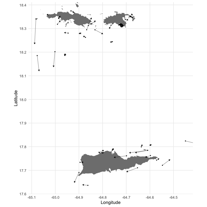
Restrict to established sites
We keep only sites first surveyed no later than 2007 (maxyearadded), so the summary reflects the established monitoring network.
Downloads
- Derived data:
s4pt6_currentsMeanMaxPulseSpeedDirectionIn2019_43sites.csv - Metadata:
s4pt6_currentsMeanMaxPulseSpeedDirectionIn2019_43sites.txt
version 1.0.0 • in-review • data ≤ 2023-12-31