Reef Code

about 2.1 Reformat raw benthic cover data 2.2 Cross-reference benthic codes 2.3 percentage cover of main benthic categories 2.4 percentage cover of coral genera 2.5 percentage cover of coral species 2.6 percentage cover of coral trait groups 2.7 percentage cover of algae taxa 2.8 percentage cover of sponge morphs 2.9 percentage cover of zoanthids and gorgonians 2.10 percentage cover of other benthic categories

internal drivers

3.1 coral health 3.2 coral interactions 3.3 fish biodiversity 3.3b fish biodiversity using NOAA data 3.4 herbivory 3.5 coral biodiversity 3.6 diadema 3.7 nuisance species

external drivers

4.1 site rugosity 4.2 site depth 4.3 site distances from shore 4.4 daily temperatures 4.5 monthly and annual DHW and temperature 4.6 currents 4.7 management 4.8 wave benthic orbital velocities pt 1 4.9 wave benthic orbital velocities pt 2 4.10 water quality 4.11 sedimentation 4.12 connectivity

resilience values

5.1 absolute and relative coral cover and diversity 5.2 resilience classification based on coral cover 5.3 benthic community: benthic organisms 5.4 NMDS of coral genera during recovery period

Reproductive Mode & RarityOlinger et al., In Review

Overview TCRMP VINPS CSUN Octocorals Interactive

2023, 2024 Bleaching EventOlinger et al. In Prep

VI Reef Resilience StudyOlinger et al. Coming Soon

(Any Others?)co-author suggestions welcome

2.3 Percentage cover of main benthic categories

Last updated

July 6, 2026

2.3 Percentage cover of main benthic categories

This page aggregates every surveyed benthic taxon into three broad functional groups used in past St. John and Caribbean benthic studies (P. Edmunds 2013; P. J. Edmunds 2002; Aronson and Precht 2000) and matched to the CSUN scheme in csun_benthicDat. The three groups are hard corals (Scleractinia and Millepora), macroalgae (fleshy and filamentous macroalgae at least 1 cm tall, for example Dictyota, Lobophora, Halimeda, Padina), and CTB (an amalgamated category combining crustose coralline algae, algal microturfs, and bare space that could not be separated in some two-dimensional imagery). We compute the annual percent cover of these three groups at each site across all three monitoring programs, then export one long-format table that downstream biodiversity, resilience, and rarity pages read.

Data sources

This page reads the benthic survey data from the TCRMP, VINPS, and CSUN monitoring programs, arriving here as benthicCoverXrefBenthicCodes.RData from the reformat and cross-reference steps (sections 2.1 and 2.2). That workspace holds the per-program benthic data frames tcrmp_benthicDat, vinps_benthicDat, and csun_random_benthicDat together with the benthicCodes cross-reference. The three programs do not share a sampling structure: TCRMP and VINPS use replicate transects, so their site-year values are transect means with a standard error, while CSUN sites carry a single quadrat-based transect per site and therefore have no replicate structure and no error bars. The derived major-benthic-category table this page produces is available in the Downloads section below.

Load workspace and define variables

We load the data written by the reformat and cross-reference steps (sections 2.1 and 2.2).

Show code

load("benthicCoverXrefBenthicCodes.RData")

subfoldername_sfg names the storage folder for the raw and cross-referenced benthic codes and stays fixed for the benthic-cover groupings. groupingvar sets how taxa are grouped on this page (here, benthicCategories). section is the naming stem for the exported output.

Show code

subfoldername_sfg <- "benthicCoverGrouped"
groupingvar <- "benthicCategories"
section <- "s2pt3" # for naming

Reorganize `benthicDat` into subgroupings of interest

We filter benthicCodes to the subgroups we want. Here we remove the Millepora category from csun_random so it does not double-count against the hard-coral group in the CSUN scheme.

Show code

benthicCodes$csun_YZTK_code[which(benthicCodes$csun_random_code == "Millepora")] <- ""

`getBenthicDatColInds()`

this is one of two functions that connect benthicDat to benthicCodes for all three programs.

getBenthicDatColInds() makes _columnInds that stores column indices of benthic codes for each benthic subgroup of interest (e.g., coral genera, coral trait groups, algae/sponge/coral/bare space)

arguments:

benthicDat is benthic dataset of interest
codecolumn is the name of the column of benthic code containing the code for benthicdat
groupingcolumn is the name of the column of benthic codes where the grouping variable of interest is stored.

Show code

getBenthicDatColInds <-
  function(benthicDat, codecolumn, groupingcolumn) {
    codecolind <-
      which(colnames(benthicCodes) == codecolumn)
    groupingcolind <-
      which(colnames(benthicCodes) == groupingcolumn)
    genusdf <-
      data.frame(group =
                   unique(benthicCodes[, groupingcolind]),
                 colinds =
                   rep(0, length(unique(benthicCodes[, groupingcolind]))))
    for (i in 1:nrow(genusdf)) {
      codei <-
        benthicCodes[which(benthicCodes[, groupingcolind] == genusdf$group[i]), ]
      genusdf$colinds[i] <-
        list(which(colnames(benthicDat) %in% codei[, codecolind]))
    }
    # UAGA-guard: warn on benthicDat data columns whose code is absent from benthicCodes and is
    # therefore silently dropped (the footgun that lost VINPS Agaricia agaricites, code UAGA).
    .known <- benthicCodes[[codecolind]]; .known <- .known[nchar(.known) > 0]
    .meta_cols <- c("program","date","site","period","replicate","replicatetype","nopts",
                    "Year","Date","SiteFullName","year","month","percentCover_allCoral",
                    "PC","Check","Notes","Transect")
    .dropped <- setdiff(colnames(benthicDat), c(.known, .meta_cols))
    if (length(.dropped) > 0)
      warning("getBenthicDatColInds(", codecolumn, "): ", length(.dropped),
              " data column(s) have codes absent from benthicCodes and are DROPPED: ",
              paste(.dropped, collapse = ", "), " -- add them to benthicCodes if they are taxa.")

    if (any(nchar(genusdf$group) == 0)) {
      genusdf <- genusdf[-which(nchar(genusdf$group) == 0), ]
    }
    
    return(genusdf)
  }

We apply getBenthicDatColInds() to each program’s _benthicDat data frame. The UAGA guard inside the function warns if any data column carries a taxon code that is absent from benthicCodes and would be silently dropped, so a render warning here flags a missing cross-reference row rather than a silent data loss.

Show code

tcrmp_columnInds <-
  getBenthicDatColInds(tcrmp_benthicDat, "tcrmp_Code", "csun_YZTK_code")
vinps_columnInds <-
  getBenthicDatColInds(vinps_benthicDat, "vinps_TaxonCode", "csun_YZTK_code")
csunrandom_columnInds <-
  getBenthicDatColInds(csun_random_benthicDat, "csun_random_code", "csun_YZTK_code")

Table 1 previews the TCRMP grouping map: each row is one benthic category and the column indices of tcrmp_benthicDat that feed it.

Show code

kbl(tcrmp_columnInds) |>
  kable_paper(full_width = F) |>
  kable_styling(
    fixed_thead = T,
    bootstrap_options = c("hover", "condensed"),
    font_size = 8
  ) |>
  scroll_box(width = "100%", height = "250px")

Sec 2.3 Table 1: TCRMP column-index map. Each benthic category and the tcrmp_benthicDat columns assigned to it (diagnostic view).

	group	colinds
2	percentCover_allCoral	8, 9, 10, 11, 12, 13, 14, 15, 16, 17, 18, 19, 22, 23, 24, 25, 26, 28, 30, 31, 32, 33, 34, 35, 36, 37, 41, 42, 43, 44, 45, 46, 48, 49, 50, 51, 52, 53, 56, 57, 58, 61, 62, 64, 65, 66, 67, 68
3	percentCover_macroalgae	95, 96, 98, 99
4	percentCover_CTB	93, 107, 108, 109, 110, 111, 112

`makeGroupedBenthicDat()`

this is the second function that connects benthicDat to benthicCodes for all three programs.

makeGroupedBenthicDat() extracts the column indices (colinds) from each row of *_columnInds.

If only one index in colinds , assigns the corresponding column from benthicdat to the i-th column of a data frame _groupedBenthicDat.

if more than one index in colinds, stores row sum of benthicDat[,colinds] in the i-th column of _groupedBenthicDat.

arguments:

benthicDat is benthic dataset of interest
columnInds is the output of getBenthicDatColInds() above that contains column indices of benthic codes for each benthic subgroup of interest

Show code

makeGroupedBenthicDat <- function(benthicDat, columnInds) {
  groupeddat <- data.frame(matrix(nrow = nrow(benthicDat),
                                  ncol = nrow(columnInds)))
  colnames(groupeddat) <- columnInds$group
  benthicDat <- benthicDat %>% dplyr::mutate(dplyr::across(dplyr::where(is.numeric), ~replace(.x, is.na(.x), 0))) 
  for (i in 1:nrow(columnInds)) {
    geni <- columnInds[i,]
    datcoli <- unlist(geni$colinds)
    if (length(datcoli) == 1) {
      groupeddat[, i] <- benthicDat[, datcoli]
    } else {
      groupeddat[, i] <- rowSums(benthicDat[, datcoli])
    }
  }
  groupeddat <- cbind(benthicDat[, 1:6], groupeddat)
  return(groupeddat)
}

We apply makeGroupedBenthicDat() to each program’s _benthicDat and its matching _columnInds.

Table 2 previews the first rows of the grouped TCRMP data: the leading survey columns followed by one percent-cover column per benthic category.

Show code

tcrmp_groupedBenthicDat <-
  makeGroupedBenthicDat(tcrmp_benthicDat, tcrmp_columnInds)
vinps_groupedBenthicDat <-
  makeGroupedBenthicDat(vinps_benthicDat, vinps_columnInds)
csun_groupedBenthicDat <-
  makeGroupedBenthicDat(csun_random_benthicDat, csunrandom_columnInds)

Show code

kbl(head(tcrmp_groupedBenthicDat)) |>
  kable_paper(full_width = F) |>
  kable_styling(
    fixed_thead = T,
    bootstrap_options = c("hover", "condensed"),
    font_size = 8
  ) |>
  scroll_box(width = "100%", height = "250px")

Sec 2.3 Table 2: Grouped TCRMP benthic data, first rows (diagnostic view). Survey columns followed by per-category percent cover.

program	date	site	period	replicate	replicatetype	percentCover_allCoral	percentCover_macroalgae	percentCover_CTB
TCRMP	2001-04-25	Cane Bay	Annual	1	transect	4.98	6.12	84.67
TCRMP	2001-04-25	Cane Bay	Annual	2	transect	26.16	2.73	66.80
TCRMP	2001-04-25	Cane Bay	Annual	3	transect	35.67	3.10	54.65
TCRMP	2001-04-25	Cane Bay	Annual	4	transect	30.43	4.71	60.15
TCRMP	2001-04-25	Cane Bay	Annual	5	transect	22.83	0.39	74.42
TCRMP	2001-04-25	Cane Bay	Annual	6	transect	15.81	10.53	67.29

Merge the `benthicDat` from three programs

We now hold three _groupedBenthicDat data frames and merge them into one. Because some benthic categories are absent from the CSUN scheme, we first align the three sets of column names so every program carries the same columns before we bind them.

First we collect the unique column names across all three data frames.

Show code

all_columns <-
  unique(c(
    colnames(tcrmp_groupedBenthicDat),
    colnames(vinps_groupedBenthicDat),
    colnames(csun_groupedBenthicDat)
  ))

Next we identify the columns missing from each data frame.

Show code

missing_columns_tcrmp <-
  setdiff(all_columns, colnames(tcrmp_groupedBenthicDat))
missing_columns_vinps <-
  setdiff(all_columns, colnames(vinps_groupedBenthicDat))
missing_columns_csung <-
  setdiff(all_columns, colnames(csun_groupedBenthicDat))

We add each missing column, filled with NA.

Show code

for (col in missing_columns_tcrmp) {
  tcrmp_groupedBenthicDat[[col]] <- NA
}
for (col in missing_columns_vinps) {
  vinps_groupedBenthicDat[[col]] <- NA
}
for (col in missing_columns_csung) {
  csun_groupedBenthicDat[[col]] <- NA
}

We reorder the columns so all three data frames share one column order.

Show code

tcrmp_groupedBenthicDat <- tcrmp_groupedBenthicDat[, all_columns]
vinps_groupedBenthicDat <- vinps_groupedBenthicDat[, all_columns]
csun_groupedBenthicDat <- csun_groupedBenthicDat[, all_columns]

We bind the aligned data frames into one groupedBenthicDat.

Show code

groupedBenthicDat <-
  rbind(tcrmp_groupedBenthicDat,
        vinps_groupedBenthicDat,
        csun_groupedBenthicDat)

We add a year column derived from the survey date.

Show code

groupedBenthicDat <- groupedBenthicDat |>
  mutate(year = lubridate::year(groupedBenthicDat$date)) |>
  relocate(year, .before = date)

We reshape groupedBenthicDat into long format, one row per site-survey-category, and drop rows with no cover value.

Show code

groupedBenthicDat <- groupedBenthicDat |>
  tidyr::gather(!!groupingvar, "perccover", 8:ncol(groupedBenthicDat))

groupedBenthicDat <- groupedBenthicDat |>
  filter(!is.na(perccover))

We add a pres column flagging whether benthicCategories was present (cover greater than zero) or absent.

Show code

groupedBenthicDat$pres <- rep(0, nrow(groupedBenthicDat))
groupedBenthicDat$pres[groupedBenthicDat$perccover > 0] <- 1

We drop the intermediate objects and keep only what the summary, plot, and export steps need.

Summarize and plot

We summarize the long-format data to an annual site-level percent cover for each benthic category. For TCRMP and VINPS the value is the transect mean with a standard error. For CSUN each site has a single quadrat-based transect, so the CSUN value carries no replicate structure and no error bar.

The summary covers 49 sites across 3 programs, spanning 1987 to 2023.

Show code

groupedBenthicDatCovSum <- groupedBenthicDat |>
  # dplyr::group_by(year, program, site, benthicCategories) |>
  dplyr::group_by(year, date, program, site, period, benthicCategories) |>
  dplyr::summarise(
    meancov = mean(perccover),
    sdcov = sd(perccover),
    secov = sd(perccover) / (sqrt(length(perccover))),
    n = length(perccover)
  )
groupedBenthicDatCovSum <- groupedBenthicDatCovSum %>% dplyr::mutate(dplyr::across(dplyr::where(is.numeric), ~replace(.x, is.na(.x), 0)))

Figure 1 shows how the three functional groups change over time at each site, with sites ordered shallow to deep so depth patterns read down the panel grid. The dashed line marks the 2005 mass bleaching year. TCRMP and VINPS panels carry a standard-error range; CSUN panels do not, because CSUN has no transect replicate.

Show code

#add site info so can plot according to increasing depth
groupedBenthicDatCovSum <-
  merge(groupedBenthicDatCovSum, sitedat, by = "site")
groupedBenthicDatCovSum <-
  groupedBenthicDatCovSum[order(groupedBenthicDatCovSum$depth), ]
groupedBenthicDatCovSum$site <- factor(groupedBenthicDatCovSum$site,
                                       levels = unique(groupedBenthicDatCovSum$site))

create_benthic_plot <- function(data,
                                x_var = "year",
                                y_var = "meancov",
                                color_var = "benthicCategories",
                                facet_var = "site",
                                error_var = "secov",
                                min_year = NULL,
                                max_year = NULL,
                                highlight_year = NULL,
                                max_facets_per_page = 35) {
  # Determine x-axis limits if not provided
  if (is.null(min_year))
    min_year <- floor(min(data[[x_var]]))
  if (is.null(max_year))
    max_year <- ceiling(max(data[[x_var]]))
  
  # Calculate optimal number of rows and columns
  n_facets <- length(unique(data[[facet_var]]))
  n_facets <- min(n_facets, max_facets_per_page)  # Limit to max_facets_per_page
  n_col <- ceiling(sqrt(n_facets))
  n_row <- ceiling(n_facets / n_col)
  
  # Create base plot
  p <- ggplot(data, aes(x = .data[[x_var]], y = .data[[y_var]], color = .data[[color_var]])) +
    geom_line() +
    geom_point(size = 1) +
    geom_linerange(aes(ymin = .data[[y_var]] - .data[[error_var]], ymax = .data[[y_var]] + .data[[error_var]]), linewidth = 0.5) +
    facet_wrap(vars(.data[[facet_var]]), nrow = n_row, ncol = n_col, scales = "free_x") +
    labs(y = "Percent cover", x = toupper(x_var)) +
    scale_y_continuous(expand = c(0, 0)) +
    scale_x_continuous(
      expand = expansion(mult = 0.04),
      breaks = seq(min_year, max_year, by = 1),
      labels = function(x)
        ifelse(x %% 5 == 0, paste0("'", substr(x, 3, 4)), "")
    ) +
    theme_bw() +
    theme(
      strip.text = element_text(size = 10),
      legend.position = "bottom",
      panel.grid = element_blank()
    )
  
  # Add highlight line if specified
  if (!is.null(highlight_year)) {
    p <- p + geom_vline(
      xintercept = highlight_year,
      color = "gray50",
      alpha = 0.5,
      linetype = "dashed"
    )
  }
  
  return(p)
}

# Usage:
stack <- create_benthic_plot(
  data = groupedBenthicDatCovSum,
  min_year = minyear,
  max_year = maxyear,
  highlight_year = 2005,
  max_facets_per_page = length(unique(groupedBenthicDatCovSum$site))
)

# Display the plot
print(stack)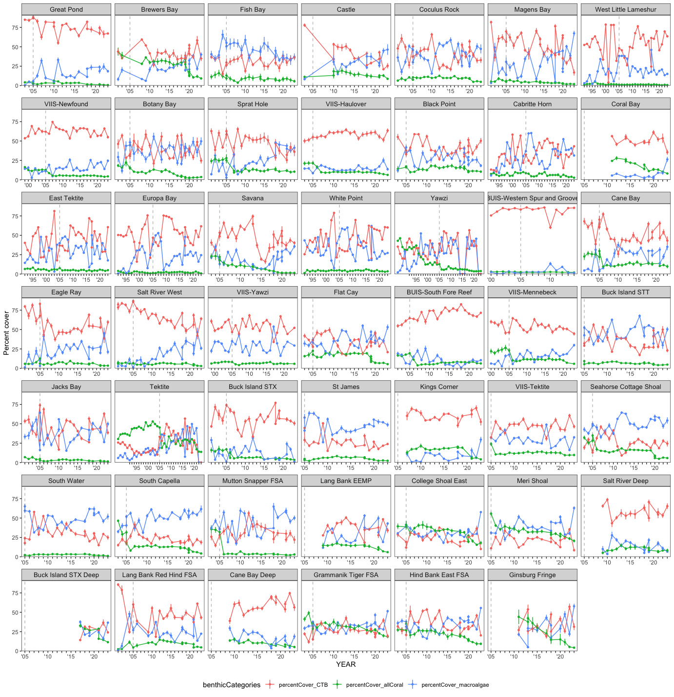

Sec 2.3 Figure 1: Percent cover of the three major benthic categories over time at each site, transect-mean plus or minus SE for TCRMP and VINPS (no error bars for CSUN, which has no transect replicate). Sites are ordered shallow to deep. The dashed line marks 2005.

Key result

Each site panel in Figure 1 carries the full recorded time series of hard-coral, macroalgae, and CTB cover on one axis. Reading the panels shallow to deep shows how the balance among the three groups shifts with depth and across the 2005 bleaching year. The underlying values are exported below for the biodiversity, resilience, and rarity pages.

Interactive dashboard

Explore the full major-benthic-category cover dataset this page produces. The plot shows mean percent cover through time for each category; the table is the complete dataset, searchable and filterable by any column.

Table shows a random sample of 15,000 of 22,980 rows. The plot above uses every row.

Downloads

The links below download the derived benthic-category table, its metadata, and this page’s source.

version 1.0.0 • in-review • data ≤ 2023

References

Aronson, Richard B., and William F. Precht. 2000. “Herbivory and Algal Dynamics on the Coral Reef at Discovery Bay, Jamaica.” Limnology and Oceanography 45 (1): 251–55. https://doi.org/10.4319/lo.2000.45.1.0251.

Edmunds, P. 2013. “Decadal-Scale Changes in the Community Structure of Coral Reefs of St. John, US Virgin Islands.” https://doi.org/10.3354/MEPS10424.

Edmunds, Peter J. 2002. “Long-Term Dynamics of Coral Reefs in St. John, US Virgin Islands.” Coral Reefs 21 (4): 357–67. https://doi.org/10.1007/s00338-002-0258-1.

2.3 Percentage cover of main benthic categories

On this page

Data sources

Load workspace and define variables

Reorganize benthicDat into subgroupings of interest

getBenthicDatColInds()

makeGroupedBenthicDat()

Merge the benthicDat from three programs

Summarize and plot

Interactive dashboard

Downloads

References

Reorganize `benthicDat` into subgroupings of interest

`getBenthicDatColInds()`

`makeGroupedBenthicDat()`

Merge the `benthicDat` from three programs