Show code
sitedat <-
  read.csv(
    "../../../RRSdata/00_RRS_dataCatalogStatus/00_RRS_siteMaster_allSites_data.csv"
)This page builds a second fish-biodiversity view of the TCRMP sites from NOAA National Coral Reef Monitoring Program (NCRMP) surveys, alongside the TCRMP transect view on page 3.3. We match each TCRMP site to the NOAA primary sample units (PSUs) that fall within it, count fish by PSU and year, and summarize species richness, abundance, and Simpson’s diversity (1/D) across sites. The site-faceted time series in Figure 1, Figure 2, Figure 3, Figure 4, and Figure 5 carry the story. The page writes two downloadable products, a per-PSU counts table and a Simpson’s diversity table, each with metadata.
This page draws on the NOAA National Coral Reef Monitoring Program fish surveys (ncrmp-fish) for the per-PSU counts and taxonomy, and on the Territorial Coral Reef Monitoring Program (tcrmp) for the trophic-group labels and the site master. A PSU-to-site crosswalk maps each TCRMP site to up to three NOAA PSUs by GPS. The NOAA survey record is filtered to 2003 through 2018, and products stay within the site embargo (data ≤ 2023). The derived per-PSU counts and Simpson’s diversity tables are available in the Downloads section below.
The site master supplies each monitoring site along with its depth and program, which the figures below use to order facets shallow to deep.
sitedat <-
read.csv(
"../../../RRSdata/00_RRS_dataCatalogStatus/00_RRS_siteMaster_allSites_data.csv"
)We read the TCRMP fish counts and keep only the annual-survey sites added by the reference year. This TCRMP table supplies the trophic-group label that we later attach to the NOAA species records.
fishcounts <-
  read.csv("../../../RRSdata/data_TCRMP/TCRMP_fishCounts_allSites_2003_2023_data.csv")
We build sitekp (sites to keep) by holding only sites added no later than the reference year, then filter fishcounts to annual surveys within the analysis window at those sites.
We drop the biomass and length columns and rename to the working schema.
The PSU-to-site crosswalk maps each site to up to three NOAA PSUs, matched from GPS coordinates in GIS. We keep only the crosswalk rows for sites in sitekp.
We read the NOAA survey .rds files (held on a private drive, not on GitHub) for the St. Thomas/St. John and St. Croix regions.
We pull the per-PSU sample data out of each region object.
STTSTJsample <- STTSTJ_2001_2021$sample_data
STXsample <- STX_2001_2021$sample_data
We restrict the NOAA survey record to 2003 through 2018.
We select the NOAA rows whose PSU matches one of the three crosswalk PSUs for each site, attaching the site name in the join.
STTSTJsample1 <- STTSTJsample |>
  filter(PRIMARY_SAMPLE_UNIT %in% sitedat_station$Sample.1) |>
  left_join(sitedat_station |> dplyr::select(site,Sample.1),
            by = c("PRIMARY_SAMPLE_UNIT" = "Sample.1"), relationship="many-to-many")

STXsample1 <- STXsample |>
  filter(PRIMARY_SAMPLE_UNIT %in% sitedat_station$Sample.1) |>
  left_join(sitedat_station |> dplyr::select(site,Sample.1),
            by = c("PRIMARY_SAMPLE_UNIT" = "Sample.1"), relationship="many-to-many")

STTSTJsample2 <- STTSTJsample |>
  filter(PRIMARY_SAMPLE_UNIT %in% sitedat_station$Sample.2) |>
  left_join(sitedat_station |> dplyr::select(site,Sample.2),
            by = c("PRIMARY_SAMPLE_UNIT" = "Sample.2"), relationship="many-to-many")

STXsample2 <- STXsample |>
  filter(PRIMARY_SAMPLE_UNIT %in% sitedat_station$Sample.2) |>
  left_join(sitedat_station |> dplyr::select(site,Sample.2),
            by = c("PRIMARY_SAMPLE_UNIT" = "Sample.2"), relationship="many-to-many")

STTSTJsample3 <- STTSTJsample |>
  filter(PRIMARY_SAMPLE_UNIT %in% sitedat_station$Sample.3) |>
  left_join(sitedat_station |> dplyr::select(site,Sample.3),
            by = c("PRIMARY_SAMPLE_UNIT" = "Sample.3"), relationship="many-to-many")

STXsample3 <- STXsample |>
  filter(PRIMARY_SAMPLE_UNIT %in% sitedat_station$Sample.3) |>
  left_join(sitedat_station |> dplyr::select(site,Sample.3),
            by = c("PRIMARY_SAMPLE_UNIT" = "Sample.3"), relationship="many-to-many")
We stack the three matched-PSU tables from both regions into one sample table.
sample <- bind_rows(STTSTJsample1,
                    STXsample1,
                    STTSTJsample2,
                    STXsample2,
                    STTSTJsample3,
                    STXsample3)
We confirm that every site-PSU pair present in the joined survey data also appears in the crosswalk, so no PSU was matched to the wrong site.
check <- sample |>
  dplyr::select(YEAR,PRIMARY_SAMPLE_UNIT,site) |>
  distinct()

check2 <- sitedat_station |>
  dplyr::select(Sample.1,Sample.2,Sample.3,site) |>
  pivot_longer(cols = c(Sample.1,Sample.2,Sample.3), names_to = "samplenum", values_to = "psu") |>
  drop_na(psu) |>
  distinct()

psu_pairs_in_sample <- nrow(dplyr::distinct(dplyr::select(check, PRIMARY_SAMPLE_UNIT, site)))
psu_pairs_matched   <- nrow(dplyr::semi_join(
  dplyr::distinct(dplyr::select(check, PRIMARY_SAMPLE_UNIT, site)),
check2, by = c("PRIMARY_SAMPLE_UNIT" = "psu", "site" = "site")))We drop the survey columns we do not use and reorder to a compact schema.
sample <- sample |> dplyr::select(-LAT_DEGREES,-LON_DEGREES, -DEPTH, -UNDERWATER_VISIBILITY, -MAPGRID_NR, -HABITAT_CD, -DEPTH_STRAT, -SUBREGION, -ADMIN, -SPECIES_NR, -TIME_SEEN, -PROT, -STRAT, -REGION)

#reorder columns
sample <- sample |>
  dplyr::select(site, YEAR, MONTH, PRIMARY_SAMPLE_UNIT,SPECIES_CD,NUM)

colnames(sample) <-
  c("site","year","month","transect","sppcode","counts")

sample <- sample |>
  filter(counts!=0)
We attach scientific and common names from the NOAA taxonomy table.
fishtaxa <- STTSTJ_2001_2021$taxonomic_data
# fishtaxa2 <- STX_2001_2021$taxonomic_data
# any(fishtaxa1 != fishtaxa2, na.rm = TRUE) # should be FALSEsample <- sample |>
left_join(fishtaxa |> select(SPECIES_CD, SCINAME, COMNAME), by = c("sppcode" = "SPECIES_CD")) |>
mutate(sppname = SCINAME) |>
mutate(commonname = COMNAME) |>
select(-SCINAME,-COMNAME) |>
relocate(counts, .after = commonname)We collapse the records to species by PSU and year, which is the unit the diversity measures use.
sample <- sample |>
  group_by(site, year, month,transect, sppname, commonname) |>
  summarize(counts = sum(counts))
We pull each species’ trophic group from the TCRMP table and attach it to the NOAA records.
tcrmp_fishsummary <- fishcounts |>
  select(sppname, commonname, trophicgroup) |>
distinct()sample <- sample |>
left_join(tcrmp_fishsummary |> select(sppname, trophicgroup), by = "sppname") |>
relocate(trophicgroup, .before = counts)The NOAA sample table now carries the same columns as the TCRMP fishcounts table on page 3.3, so the rest of the page reuses that name.
fishcounts <- sampleWe summarize richness and abundance per PSU and per site, both overall and by trophic group. The site-level summaries carry the mean and standard deviation across PSUs, which feed the ribbon envelopes in the figures.
fishsum_troph <- fishcounts |>
  group_by(year, site, transect, trophicgroup) |>
  summarise(diversity = length(unique(sppname)),
            counts = sum(counts))

fishsum_trophsum <- fishsum_troph |>
  group_by(year, site, trophicgroup) |>
  summarise(
    meandiv = mean(diversity),
    sddiv = sd(diversity),
    meancounts = mean(counts),
    sdcounts = sd(counts)
  )

fishsum_tot <- fishcounts |>
  group_by(year, site, transect) |>
  summarise(diversity = length(unique(sppname)),
            counts = sum(counts))

fishsum_totsum <- fishsum_tot |>
  group_by(year, site) |>
  summarise(
    meandiv = mean(diversity),
    sddiv = sd(diversity),
    meancounts = mean(counts),
    sdcounts = sd(counts)
  )
Before plotting, we order the sites shallow to deep so each faceted panel reads from reef flat to depth. The NOAA surveys carry replicate PSUs at each site, so the mean and standard deviation across PSUs support the ribbon envelope shown here. The dashed line marks the 2005 Caribbean bleaching year.
Figure 1 shows annual mean species richness at each site, with the shaded band spanning one standard deviation across PSUs.
fishsum_totsum <-
  merge(fishsum_totsum, sitedat, by = "site")
fishsum_totsum <-
  fishsum_totsum[order(fishsum_totsum$depth),]

fishsum_totsum$site <- factor(fishsum_totsum$site,
                              levels = unique(fishsum_totsum$site))

ggplot(
  fishsum_totsum,
  aes(
    x = year,
    y = meandiv,
    fill = depth,
    ymin = meandiv - sddiv,
    ymax = meandiv + sddiv
  )
) +
  scale_fill_continuous(low = "red", high = "blue") +
  scale_x_continuous(labels = function(x) ifelse(x %% 5 == 0, paste0("'", substr(x, 3, 4)), "")) +
  facet_wrap(. ~ site , scales = "fixed") +
  geom_ribbon(alpha = .5) +
  geom_line(size = 0.25) +
  geom_point(size = 0.5) +
  xlab("year") +
  ylab("species richness") +
  geom_vline(
    xintercept = 2005,
    color = "gray50",
    alpha = 0.5,
    lty = "dashed"
  ) +
  theme_bw() +
  theme(strip.text = element_text(size = 9)) +
  theme(legend.position = "bottom") +
  theme(panel.grid.major = element_blank(),
        panel.grid.minor = element_blank())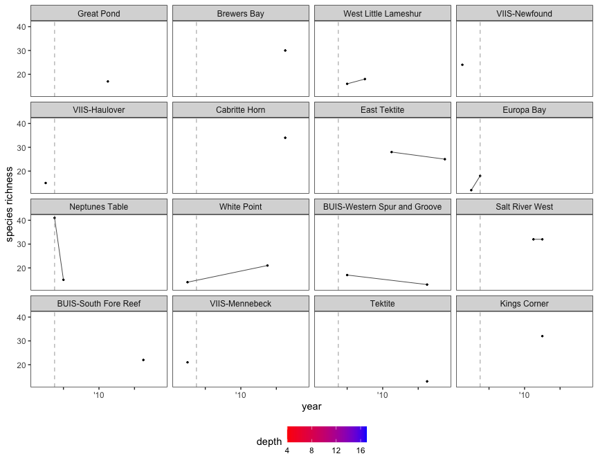
Figure 2 shows annual mean fish abundance (individuals counted) at each site.
ggplot(
  fishsum_totsum,
  aes(
    x = year,
    y = meancounts,
    fill = depth,
    ymin = meancounts - sdcounts,
    ymax = meancounts + sdcounts
  )
) +
  scale_fill_continuous(low = "red", high = "blue") +
  scale_x_continuous(labels = function(x) ifelse(x %% 5 == 0, paste0("'", substr(x, 3, 4)), "")) +
  facet_wrap(. ~ site , scales = "fixed") +
  geom_ribbon(alpha = .5) +
  geom_line(size = 0.25) +
  geom_point(size = 0.5) +
  xlab("year") +
  ylab("abundance (# individuals)") +
  geom_vline(
    xintercept = 2005,
    color = "gray50",
    alpha = 0.5,
    lty = "dashed"
  ) +
  theme_bw() +
  theme(strip.text = element_text(size = 9)) +
  theme(legend.position = "bottom") +
  theme(panel.grid.major = element_blank(),
        panel.grid.minor = element_blank())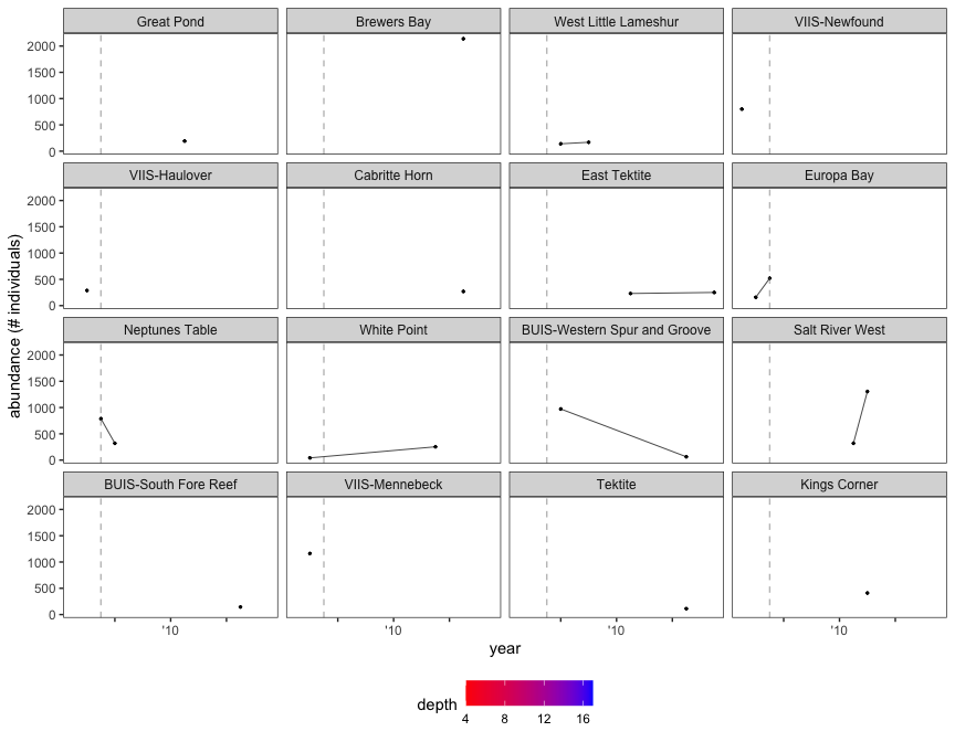
Figure 3 splits species richness by trophic group, so each site panel shows how many species from each feeding guild were recorded over time.
fishsum_trophsum <-
  merge(fishsum_trophsum, sitedat, by = "site")
fishsum_trophsum <-
  fishsum_trophsum[order(fishsum_trophsum$depth),]
fishsum_trophsum$site <- factor(fishsum_trophsum$site,
                                levels = unique(fishsum_trophsum$site))

ggplot(
  fishsum_trophsum,
  aes(
    x = year,
    y = meandiv,
    color = trophicgroup,
    fill = trophicgroup,
    ymin = meandiv - sddiv,
    ymax = meandiv + sddiv
  )
) +
  scale_x_continuous(labels = function(x) ifelse(x %% 5 == 0, paste0("'", substr(x, 3, 4)), "")) +
  facet_wrap(. ~ site , scales = "fixed") +
  geom_ribbon(alpha = 0.25, linewidth = 0) +
  geom_line(size = 0.25) +
  geom_point(size = 0.5) +
  xlab("year") +
  ylab("species richness") +
  geom_vline(
    xintercept = 2005,
    color = "gray50",
    alpha = 0.5,
    lty = "dashed"
  ) +
  theme_bw() +
  theme(strip.text = element_text(size = 9)) +
  theme(legend.position = "bottom") +
  theme(panel.grid.major = element_blank(),
        panel.grid.minor = element_blank())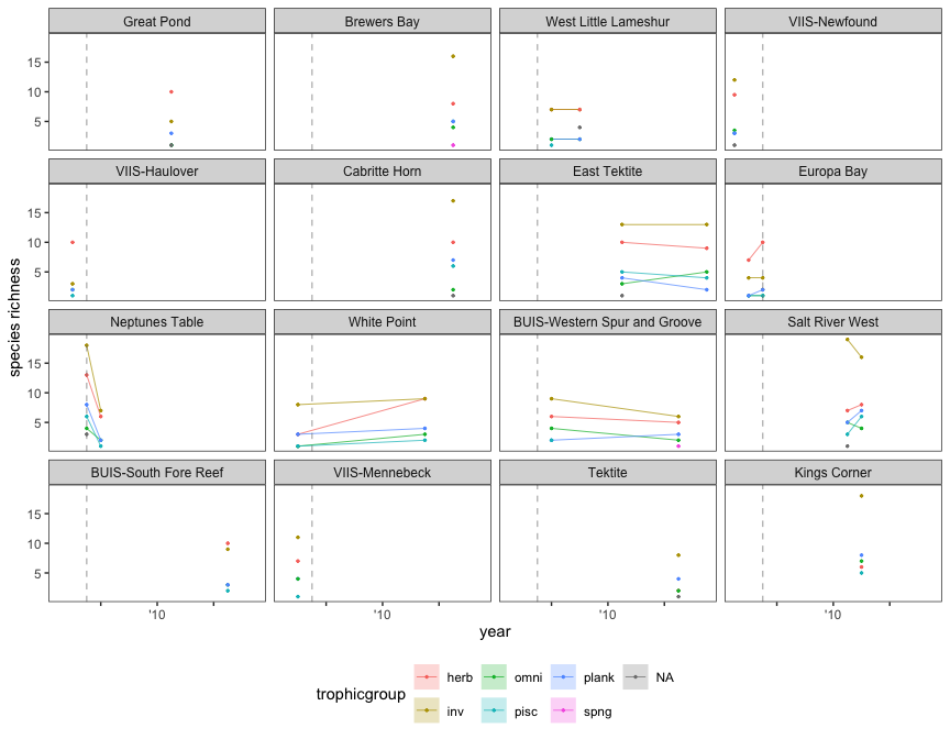
Figure 4 splits abundance by trophic group. The y-axis is capped at 800 individuals to keep the trends readable across sites.
ggplot(
  fishsum_trophsum,
  aes(
    x = year,
    y = meancounts,
    color = trophicgroup,
    fill = trophicgroup,
    ymin = meancounts - sdcounts,
    ymax = meancounts + sdcounts
  )
) +
  scale_x_continuous(labels = function(x) ifelse(x %% 5 == 0, paste0("'", substr(x, 3, 4)), "")) +
  facet_wrap(. ~ site , scales = "fixed") +
  geom_ribbon(alpha = 0.25, linewidth = 0) +
  geom_line(size = 0.25) +
  geom_point(size = 0.5) +
  xlab("year") +
  ylab("abundance (# individuals)") +
  coord_cartesian(ylim = c(0, 800)) +
  geom_vline(
    xintercept = 2005,
    color = "gray50",
    alpha = 0.5,
    lty = "dashed"
  ) +
  theme_bw() +
  theme(strip.text = element_text(size = 9)) +
  theme(legend.position = "bottom") +
  theme(panel.grid.major = element_blank(),
        panel.grid.minor = element_blank())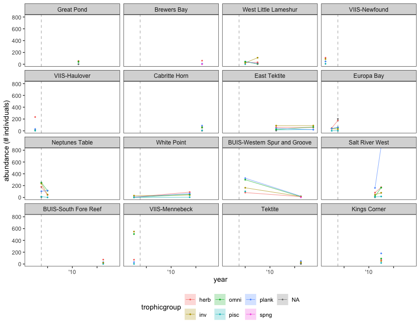
Simpson’s index considers both species richness and evenness, like the Shannon-Wiener index. We compute it per PSU and year, then report the diversity form 1/D.
\[ D = \sum_{i=1}^{S} p_i^2 \]
Here \(p_i\) is the proportion of individuals of species \(i\) and \(S\) is the number of species. A higher \(D\) means lower diversity, so we report the reciprocal \(1/D\), which increases with diversity.
simpson_calculation <- fishcounts |>
  group_by(site, year, month, transect) |>
  summarise(total = sum(counts))  |>
  left_join(fishcounts)  |>
  mutate(proportion = counts / total) |>
  group_by(site, year, month, transect)  |>
  summarise(simpson_index = sum(proportion ^ 2))  |>
  mutate(simpson_diversity = 1 / simpson_index)

simpson_calculation_sum <- simpson_calculation |>
  group_by(site, year) |>
  summarise(meandiv = mean(simpson_diversity),
            sddiv = sd(simpson_diversity))
Figure 5 shows annual mean Simpson’s diversity (1/D) at each site, with the ribbon spanning one standard deviation across PSUs.
simpson_calculation_sum <-
  merge(simpson_calculation_sum, sitedat, by = "site")
simpson_calculation_sum <-
  simpson_calculation_sum[order(simpson_calculation_sum$depth),]

simpson_calculation_sum$site <- factor(simpson_calculation_sum$site,
                                       levels = unique(simpson_calculation_sum$site))

p <-
  ggplot(
    simpson_calculation_sum,
    aes(
      x = year,
      y = meandiv,
      fill = depth,
      ymin = meandiv - sddiv,
      ymax = meandiv + sddiv
    )
  ) +
  scale_fill_continuous(low = "red", high = "blue") +
  scale_x_continuous(labels = function(x) ifelse(x %% 5 == 0, paste0("'", substr(x, 3, 4)), "")) +
  facet_wrap(. ~ site , scales = "fixed") +
  geom_ribbon(alpha = .5) +
  geom_line(size = 0.25) +
  geom_point(size = 0.5) +
  xlab("year") +
  ylab("Simpson's diversity (1/D)") +
  geom_vline(
    xintercept = 2005,
    color = "gray50",
    alpha = 0.5,
    lty = "dashed"
  ) +
  theme_bw() +
  theme(strip.text = element_text(size = 9)) +
  theme(legend.position = "bottom") +
  theme(panel.grid.major = element_blank(),
        panel.grid.minor = element_blank())

p

# svg(filename="fishdiv.svg", width = 13, height =13)
# p
# dev.off()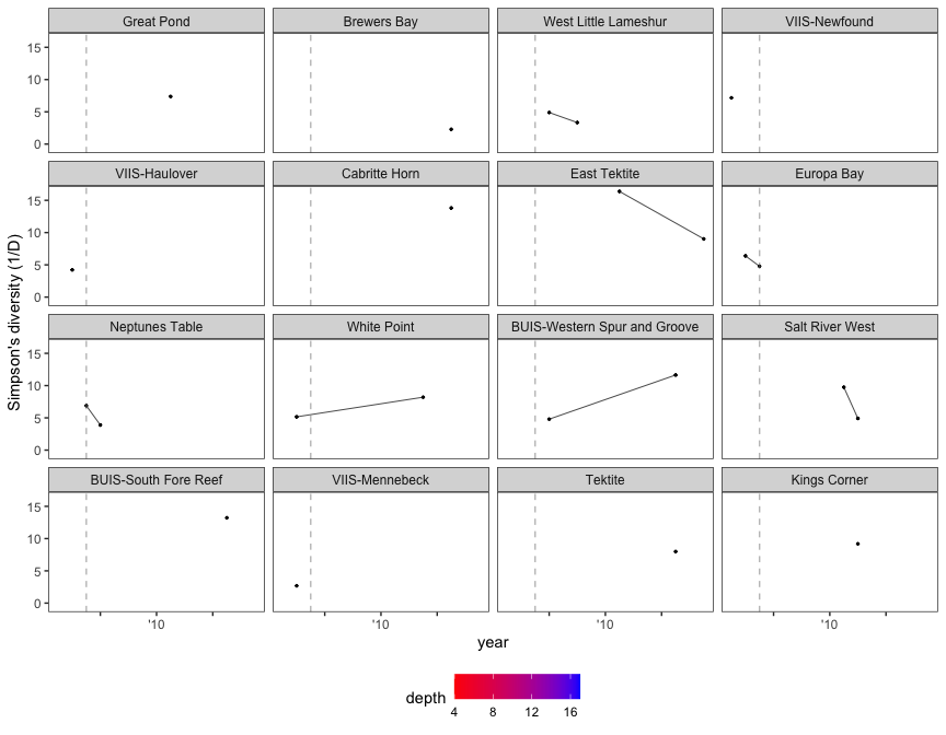
This page writes two products to outputs/: the per-PSU fish counts (fishbiodivCountsNOAA) and the Simpson’s diversity table (fishbiodivSimpsonsNOAA), each with a metadata sidecar. The filenames carry the section tag, site count, and year range.
s3pt3b_fishbiodivCountsNOAA_16sites_2003_2017.csvs3pt3b_fishbiodivCountsNOAA_16sites_2003_2017.txts3pt3b_fishbiodivSimpsonsNOAA_16sites_2003_2017.csvs3pt3b_fishbiodivSimpsonsNOAA_16sites_2003_2017.txtversion 1.0.0 • in-review • data ≤ 2023-12-31