Reef Code

About Analyses Outputs

About this site

Data Sources

more about

study sites making of the logo

benthic cover

about 2.1 Reformat raw benthic cover data 2.2 Cross-reference benthic codes 2.3 percentage cover of main benthic categories 2.4 percentage cover of coral genera 2.5 percentage cover of coral species 2.6 percentage cover of coral trait groups 2.7 percentage cover of algae taxa 2.8 percentage cover of sponge morphs 2.9 percentage cover of zoanthids and gorgonians 2.10 percentage cover of other benthic categories

internal drivers

3.1 coral health 3.2 coral interactions 3.3 fish biodiversity 3.3b fish biodiversity using NOAA data 3.4 herbivory 3.5 coral biodiversity 3.6 diadema 3.7 nuisance species

external drivers

4.1 site rugosity 4.2 site depth 4.3 site distances from shore 4.4 daily temperatures 4.5 monthly and annual DHW and temperature 4.6 currents 4.7 management 4.8 wave benthic orbital velocities pt 1 4.9 wave benthic orbital velocities pt 2 4.10 water quality 4.11 sedimentation 4.12 connectivity

resilience values

5.1 absolute and relative coral cover and diversity 5.2 resilience classification based on coral cover 5.3 benthic community: benthic organisms 5.4 NMDS of coral genera during recovery period

Reproductive Mode & RarityOlinger et al., In Review

Overview TCRMP VINPS CSUN Octocorals Interactive

2023, 2024 Bleaching EventOlinger et al. In Prep

VI Reef Resilience StudyOlinger et al. Coming Soon

(Any Others?)co-author suggestions welcome

3.4 Herbivory

3.4 Herbivory

On this page

This page estimates parrotfish herbivory on TCRMP reefs and shows how herbivore abundance, biomass, and grazing intensity vary across sites over time. The workflow keeps the seven Scarus and Sparisoma species with published bite parameters, converts counts to biomass with species length-weight coefficients, and applies the bite-rate and bite-size equations of Mumby (2006) to compute the proportion of reef grazed per hour at each site. It produces four site-faceted time series (abundance, biomass, grazing intensity by site, and annual mean grazing intensity), each with a dashed reference line at the 2005 Caribbean-wide bleaching year, and one downloadable data product with matching metadata. The abundance and biomass conversions cover Scarus and Sparisoma only, so this page describes parrotfish grazing rather than total herbivory.

Data sources

This page reads the TCRMP annual fish transect counts and the TCRMP site master, both from the TCRMP program, and the published parrotfish bite-rate, bite-size, and length-weight parameters described under herbivory parameters. The bite-rate and bite-size parameters exist for Scarus and Sparisoma only, and transect area changed over the record (60 m² before 2009, 100 m² from 2009 onward), which the grazing calculation accounts for. The derived per-transect counts, biomass, and grazing intensities computed here are available in the Downloads section below.

Site data

The site master lists each monitoring site with its island, depth, and the year it was added.

sitedat <-
  read.csv(
    "../../../RRSdata/00_RRS_dataCatalogStatus/00_RRS_siteMaster_allSites_data.csv"
  )

Load the fish counts

What happens here: the page reads the raw TCRMP annual fish transect counts, the input for every biomass and grazing calculation below.

fishcounts <-
  read.csv(
    "../../../RRSdata/data_TCRMP/TCRMP_fishCounts_allSites_2003_2023_data.csv"
  )

An optional site-and-year filter (keep annual surveys within the embargo window, and sites added no later than 2003) is kept below for reference. It is commented out, so the current run uses the full fish-count file as loaded.

# sitekp <-
#   sitedat |>
#   filter(program == "TCRMP" &
#            yearadded <= maxyearadded) |>
#   select(site)
#
# fishcounts <-
#   fishcounts |>
#   filter(Period == "Annual") |>
#   filter(SampleYear >= minyear &
#            SampleYear <= maxyear) |>
#   filter(Location %in% sitekp$site)

Bite-size and bite-rate constants

The bite-size equation uses a multiplier from Bruggemann et al. (1996).

bitesizemultiplyer = 0.0001

The genus and species tables hold the bite-rate and bite-size parameters for Scarus and Sparisoma (Mumby 2006; Bruggemann et al. 1996).

genusinfo <- data.frame(
  genus = c("Sparisoma", "Scarus"),
  w = c(1, 1),
  biterateparama = c(1088, 3329),
  biterateparamb = c(17.12, 33),
  bitesizeparamm = c(5.839, 4.013)
)

speciesinfo <- data.frame(
  species = c(
    "Scarus vetula",
    "Scarus taeniopterus",
    "Scarus iserti",
    "Sparisoma aurofrenatum",
    "Sparisoma rubripinne",
    "Sparisoma chrysopterum",
    "Sparisoma viride"
  ),
  offset = c(0,
             1196,
             1714,
             260,
             142,
             264,
             56)
)

The forklengths table records the median fork length for each size bin. The fish counts store size bins as range column names like “10-20”, so the code splits each range and takes its midpoint. The table holds two columns: the size bin and its median length.

sizebins <- colnames(fishcounts[, 9:19])
sizebins <- gsub("X", "", sizebins)
sizebins <- gsub("\\.", "-", sizebins)

forklengths <-
  data.frame(sizebin = sizebins,
             median = unlist(lapply(lapply(
               strsplit(sizebins, "-"), as.numeric
             ), median)))

forklengths$median[2:length(forklengths$median)] <-
  forklengths$median[2:length(forklengths$median)] - 0.5 # to match capstone median values  

Keep only the parrotfish species with known bite parameters, then reshape the size-bin columns into a tidy long form.

fishcounts <- fishcounts |>
  filter(ScientificName %in% speciesinfo$species) |>
  select(colnames(fishcounts[, 1:19])) |>
  # as.data.frame()|>
  pivot_longer(
    cols = colnames(fishcounts[, 9:19]),
    names_to = "sizebin",
    values_to = "counts"
  ) |>
  arrange(Location,
          SampleYear,
          SampleMonth,
          Period,
          Transect,
          ScientificName,
          sizebin)

Clean the size-bin labels and rename the columns to short, consistent names.

fishcounts$sizebin <- gsub("X", "", fishcounts$sizebin)
fishcounts$sizebin <- gsub("\\.", "-", fishcounts$sizebin)

colnames(fishcounts) <- c(
  "site",
  "year",
  "month",
  "period",
  "transect",
  "sppname",
  "commonname",
  "trophicgroup",
  "sizebin",
  "counts"
)

Join each record to its median fork length from forklengths.

fishcounts <-
  merge(forklengths, fishcounts, by = "sizebin", sort = T)

Biomass conversions

The speciessizeconversions table holds the length-weight coefficients (a and b) for each herbivore species. It comes from the 2020 capstone folder file “Copy of Biomass_Size_Conversions.csv”.

speciessizeconversions <- data.frame(
  sppname = c(
    "Acanthurus bahianus",
    "Acanthurus chirurgus",
    "Acanthurus coeruleus",
    "Kyphosus sectatrix",
    "Microspathodon chrysurus",
    "Scarus coelestinus",
    "Scarus coelruleus",
    "Scarus guacamaia",
    "Scarus iserti",
    "Scarus taeniopterus",
    "Scarus vetula",
    "Sparisoma atomarium",
    "Sparisoma aurofrenatum",
    "Sparisoma chrysopterum",
    "Sparisoma radians",
    "Sparisoma rubripinne",
    "Sparisoma viride",
    "Stegastes adustus",
    "Stegastes diencaeus",
    "Stegastes leucostictus",
    "Stegastes partitus",
    "Stegastes planifrons",
    "Stegastes variabilis"
  ),
  a = c(
    0.0237,
    0.004,
    0.0415,
    0.0174,
    0.0239,
    0.0153,
    0.0124,
    0.0155,
    0.0147,
    0.0335,
    0.025,
    0.0121,
    0.0046,
    0.0099,
    0.0162,
    0.0156,
    0.025,
    0.0349,
    0.0349,
    0.0349,
    0.0349,
    0.0349,
    0.0349
  ),
  b = c(
    2.9752,
    3.5328,
    2.8346,
    3.08,
    3.0825,
    3.0618,
    3.1109,
    3.0626,
    3.0548,
    2.7086,
    2.9214,
    3.0275,
    3.4291,
    3.1708,
    3.0252,
    3.0641,
    2.9214,
    2.9109,
    2.9109,
    2.9109,
    2.9109,
    2.9109,
    2.9109
  )
)

The biomass calculation follows the methods of Williams and Polunin (2001) and Marks and Klomp (2003). For each herbivore species, the code raises the median fork length of the size bin to the power b, multiplies by a, and multiplies by the observed count. The coefficients a and b come from linear regression of log-transformed length-weight data (Bohnsack and Harper, 1988).

The biomass formula is:

Biomass (X) = median^b * a * counts

What happens here: the loop applies this formula to every record in fishcounts and stores the result in a new biomass column.

fishcounts$biomass <- 0
for (i in 1:nrow(fishcounts)) {
  indi <- fishcounts[i, ]
  conv <-
    speciessizeconversions[which(speciessizeconversions$sppname == indi$sppname),]
  fishcounts$biomass[i] <- (indi$median ^ conv$b) * conv$a * indi$counts
}

Summarize for plotting

Summarize herbivore abundance and biomass into herbsummary, first summing across size classes within each transect, then averaging across transects for each site and year.

# first sum biomass and  counts across size classes
herbsummary <- fishcounts |>
  filter(period == "Annual") |>
  group_by(trophicgroup, sppname, commonname, year, site, transect) |>
  summarise(biomass = sum(biomass),
            counts = sum(counts))

#then average biomass and counts across years and sites
herbsummary <- herbsummary |>
  group_by(trophicgroup, sppname, commonname, year, site) |>
  summarise(
    meanbiomass = mean(biomass),
    sdbiomass = sd(biomass),
    nbiomass = length(biomass),
    meancounts = mean(counts),
    sdcounts = sd(counts),
    ncounts = length(counts)
  )

Add the site depth so facets can be ordered shallow to deep.

herbsummary <-
  merge(herbsummary, sitedat, by = "site")
herbsummary <-
  herbsummary[order(herbsummary$depth),]

herbsummary$site <- factor(herbsummary$site,
                           levels = unique(herbsummary$site))

herbsummary$sppname <- factor(herbsummary$sppname,
                              levels = unique(herbsummary$sppname))

Figure 1 stacks mean parrotfish abundance by species at each TCRMP site, with facets ordered shallow to deep and a dashed line at the 2005 bleaching year.

ggplot(herbsummary,
       aes(
         x = year,
         y = meancounts,
         color = sppname,
         fill = sppname,
         group = sppname
       )) +
  facet_wrap(~ site) +
  geom_area(position = 'stack', alpha = 0.5) +
  # geom_point(position = 'stack') +
  # geom_line(position = 'stack') +
  ylab("counts") +
  scale_y_continuous(expand = c(0, 0)) +
  geom_vline(
    xintercept = 2005,
    color = "gray50",
    alpha = 0.5,
    lty = "dashed"
  ) +
  # theme_classic() +
  theme(strip.text = element_text(size = 10)) +
  theme(legend.position = "bottom") +
  theme(panel.grid.major = element_blank(),
        panel.grid.minor = element_blank())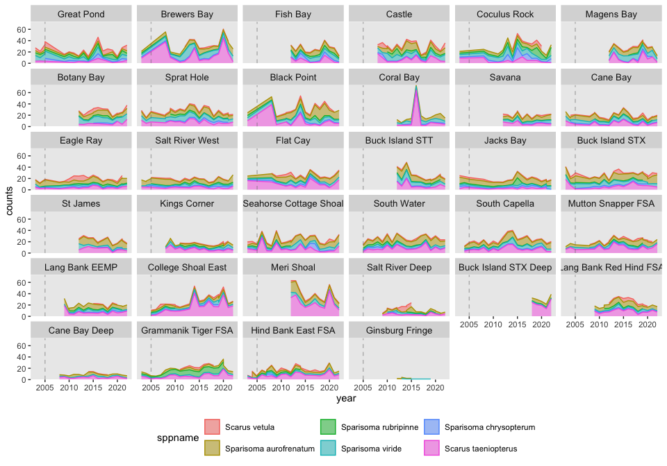

Sec 3.4 Figure 1: Mean herbivore abundance (counts) by species across TCRMP sites, ordered shallow to deep. Dashed line marks the 2005 Caribbean-wide bleaching year.

Figure 2 shows the same site-faceted series for biomass, so heavier-bodied species contribute more than they do to the abundance view.

ggplot(herbsummary,
       aes(
         x = year,
         y = meanbiomass,
         color = sppname,
         fill = sppname,
         group = sppname
       )) +
  facet_wrap(~ site) +
  geom_area(position = 'stack', alpha = 0.5) +
  # geom_point(position = 'stack') +
  # geom_line(position = 'stack') +
  ylab("biomass") +
  scale_y_continuous(expand = c(0, 0)) +
  geom_vline(
    xintercept = 2005,
    color = "gray50",
    alpha = 0.5,
    lty = "dashed"
  ) +
  # theme_classic() +
  theme(strip.text = element_text(size = 10)) +
  theme(legend.position = "bottom") +
  theme(panel.grid.major = element_blank(),
        panel.grid.minor = element_blank())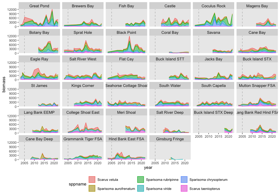

Sec 3.4 Figure 2: Mean herbivore biomass (g) by species across TCRMP sites, ordered shallow to deep. Dashed line marks the 2005 Caribbean-wide bleaching year.

Bite rate, bite size, and grazing calculations

What happens here: the next chunks define the bite-rate and bite-size functions from Mumby (2006), apply them to every record, and combine them with counts and transect area to derive the proportion of reef grazed per hour.

The biterate function returns the bites per hour for one record, from the genus and species parameters.

biterate <- function(x) {
  ind <- fishcounts[x, ]
  if (ind$counts > 0) {
    gi <-
      genusinfo[which(genusinfo$genus == strsplit(ind$sppname, " ")[[1]][1]), ]
    si <- speciesinfo[which(speciesinfo$species == ind$sppname), ]
    fi <- forklengths[which(forklengths$sizebin == ind$sizebin), ]
    r <-
      gi$w * (gi$biterateparama - (gi$biterateparamb * fi$median) - si$offset)
  } else {
    r = 0
  }
  return(r)
}

The bitesize function returns the area of one bite for the record, scaled by fork length.

bitesize <- function(x) {
  ind <- fishcounts[x, ]
  if (ind$counts > 0) {
    gi <-
      genusinfo[which(genusinfo$genus == strsplit(ind$sppname, " ")[[1]][1]), ]
    fi <- ind$median
    m <- gi$bitesizeparamm * bitesizemultiplyer * (fi ^ 2)
  } else {
    m = 0
  }
  return(m)
}

Populate the bite-rate and bite-size columns for every record (eq. 2-3 in Mumby (2006)).

fishcounts$biterate <-
  vapply(1:nrow(fishcounts), function(i)
    biterate(i), numeric(1))
fishcounts$bitesize <-
  vapply(1:nrow(fishcounts), function(i)
    bitesize(i), numeric(1))

Multiply counts, bite rate, and bite size for each species and size class to get the area grazed by that group on the transect (part of eq. 4 in Mumby (2006)).

fishcounts$prod <-
  fishcounts$counts * fishcounts$biterate * fishcounts$bitesize

Sum the area grazed across species and size classes for each transect and year (rest of eq. 4 in Mumby (2006)).

fishcounts_peryear_transect <- fishcounts |>
  group_by(site, year, transect) |>
  summarise(
    tg = sum(prod),
    biomass = sum(biomass),
    counts = sum(counts)
  )

Set the surveyed transect area: 60 m² before 2009 and 100 m² from 2009 onward.

fishcounts_peryear_transect$ta <- 100
fishcounts_peryear_transect$ta[which(fishcounts_peryear_transect$year < 2009)] <-
  60

Calculate g, the percentage of the reef area grazed per hour, for each transect and year (eq. 5 in Mumby (2006)).

fishcounts_peryear_transect$g <-
  (fishcounts_peryear_transect$tg / 10000) * (1 / fishcounts_peryear_transect$ta) *
  100

Average g across transects to get an annual mean per site.

fishcounts_peryear <- fishcounts_peryear_transect |>
  group_by(site, year) |>
  summarise (
    gmean = mean(g),
    gsd = sd(g),
    gse = sd(g) / sqrt(length(g))
  )

Average g across years to get one site-level mean.

fishcounts_siteave <- fishcounts_peryear_transect |>
  group_by(site) |>
  summarise (
    gmean = mean(g),
    gsd = sd(g),
    gse = sd(g) / sqrt(length(g))
  )

Plot grazing rates

Add the site depth to each grazing table so the figures can be ordered shallow to deep.

fishcounts_peryear_transect <-
  merge(fishcounts_peryear_transect, sitedat, by = "site")
fishcounts_peryear_transect <-
  fishcounts_peryear_transect[order(fishcounts_peryear_transect$depth),]

fishcounts_peryear_transect$site <-
  factor(fishcounts_peryear_transect$site,
         levels = unique(fishcounts_peryear_transect$site))

fishcounts_peryear <-
  merge(fishcounts_peryear, sitedat, by = "site")
fishcounts_peryear <-
  fishcounts_peryear[order(fishcounts_peryear$depth),]

fishcounts_peryear$site <- factor(fishcounts_peryear$site,
                                  levels = unique(fishcounts_peryear$site))

fishcounts_siteave <-
  merge(fishcounts_siteave, sitedat, by = "site")
fishcounts_siteave <-
  fishcounts_siteave[order(fishcounts_siteave$depth),]

fishcounts_siteave$site <- factor(fishcounts_siteave$site,
                                  levels = unique(fishcounts_siteave$site))

Figure 3 compares grazing intensity across sites, ordered by depth, with the site mean and standard deviation over each year’s transect values. The comparable capstone figure used a 2007-2017 window, so the year range here differs.

boxp <- ggplot() +
  geom_jitter(
    data = fishcounts_peryear_transect,
    aes(x = site, y = g, color =
          year),
    size = 1.4,
    width = 0.2
  ) +
  scale_color_continuous(low = "magenta", high = "lightblue") +
  # geom_boxplot(data = fishcounts_peryear_transect, aes(x = site, y = g), alpha =
  #                0.2, linewidth=1.5) +
  scale_x_discrete(limits = rev) +
  geom_point(data = fishcounts_siteave,
             aes(x = site, y = gmean),
             col =
               "black",
             size = 2) +
  geom_errorbar(
    data = fishcounts_siteave,
    aes(
      x = site,
      ymax = gmean + gsd,
      ymin = gmean - gsd
    ),
    col = "black",
    linewidth = 1
  ) +
  ylab("grazing intensity (prop. reef grazed/h)") +
  theme_bw() +
  coord_flip(ylim = c(0, 1)) +
  scale_y_continuous(expand = c(0, 0)) +
  theme(legend.position = "bottom")
boxp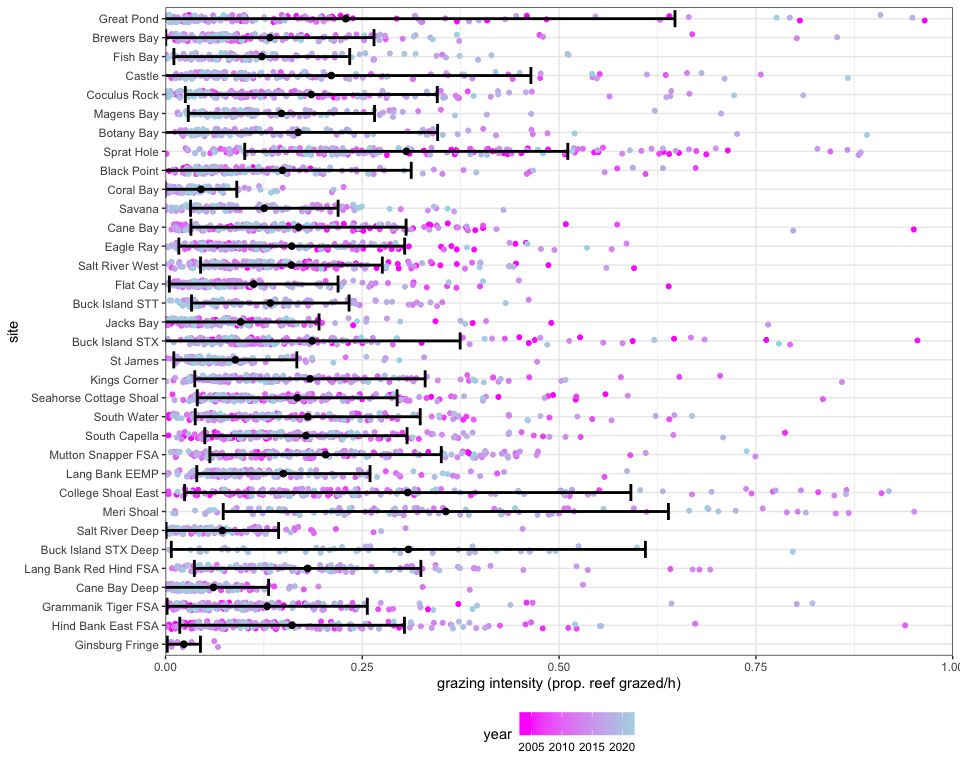

Sec 3.4 Figure 3: Grazing intensity (proportion of reef grazed per hour) across TCRMP sites, ordered by depth. Black point is the site mean with lines showing +/- 1 SD; background points are colored by year.

Figure 4 tracks the annual mean grazing intensity at each site over time, with facets ordered shallow to deep.

p <-
  ggplot(
    fishcounts_peryear,
    aes(
      x = year,
      y = gmean,
      fill = depth,
      ymin = gmean - gsd,
      ymax = gmean + gsd
    )
  ) +
  scale_fill_continuous(low = "red", high = "blue") +
  facet_wrap(. ~ site , scales = "fixed") +
  geom_ribbon(alpha = .5) +
  geom_line(size = 0.25) +
  geom_point(size = 0.5) +
  ylab("grazing intensity (prop. reef grazed/h)") +
  coord_cartesian(ylim = c(0, 1)) +
  # scale_y_continuous(expand = c(0, 0)) +
  geom_vline(
    xintercept = 2005,
    color = "gray50",
    alpha = 0.5,
    lty = "dashed"
  ) +
  theme_bw() +
  theme(strip.text = element_text(size = 10)) +
  theme(legend.position = "bottom") +
  theme(panel.grid.major = element_blank(),
        panel.grid.minor = element_blank())

p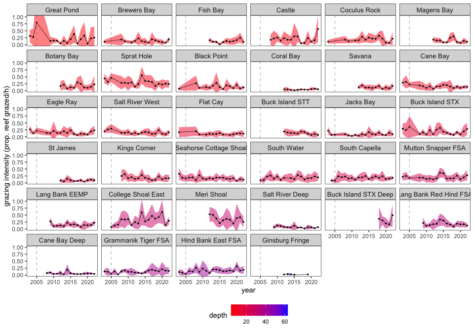

Sec 3.4 Figure 4: Annual mean herbivore grazing intensity (proportion of reef grazed per hour) across TCRMP sites, ordered shallow to deep. Ribbon shows +/- 1 SD; dashed line marks the 2005 bleaching year.

TipShiny concept: parrotfish grazing explorer

• Purpose: let a reader browse parrotfish grazing at one site at a time, instead of reading every facet at once.
• Data: herbivoreCountsBiomassGrazingintensity (the per-transect product this page writes).
• Controls: a site picker (ordered shallow to deep), a metric toggle (abundance, biomass, or grazing intensity), and a year-range slider.
• Main output: a single time-series panel for the chosen site and metric, with the 2005 reference line and the transect spread.
• Value: the four site-faceted figures here are dense; a per-site view is easier to read and to compare across depths.
• Priority: medium.

Downloads

This page writes one data product, the per-transect herbivore counts, biomass, and grazing intensities, with its metadata sidecar.

NoteDownload

• Derived data: s3pt4_herbivoreCountsBiomassGrazingintensity_34sites_2003_2022.csv
• Metadata: s3pt4_herbivoreCountsBiomassGrazingintensity_34sites_2003_2022.txt

---

version 1.0.0 • in-review • data ≤ 2023-12-31

References

Bruggemann, J. H., A. V. Kessel, V. Rooij, and A. Breeman. 1996. “Bioerosion and Sediment Ingestion by the Caribbean Parrotfish Scarus Vetula and Sparisoma Viride: Implications of Fish Size, Feeding Mode and Habitat Use.” https://doi.org/10.3354/MEPS134059.

Mumby, Peter J. 2006. “The impact of exploiting grazers (Scaridae) on the dynamics of Caribbean coral reefs.” Ecological Applications: A Publication of the Ecological Society of America 16 (2): 747–69. https://doi.org/10.1890/1051-0761(2006)016[0747:tioegs]2.0.co;2.