Reef Code

about 2.1 Reformat raw benthic cover data 2.2 Cross-reference benthic codes 2.3 percentage cover of main benthic categories 2.4 percentage cover of coral genera 2.5 percentage cover of coral species 2.6 percentage cover of coral trait groups 2.7 percentage cover of algae taxa 2.8 percentage cover of sponge morphs 2.9 percentage cover of zoanthids and gorgonians 2.10 percentage cover of other benthic categories

internal drivers

3.1 coral health 3.2 coral interactions 3.3 fish biodiversity 3.3b fish biodiversity using NOAA data 3.4 herbivory 3.5 coral biodiversity 3.6 diadema 3.7 nuisance species

external drivers

4.1 site rugosity 4.2 site depth 4.3 site distances from shore 4.4 daily temperatures 4.5 monthly and annual DHW and temperature 4.6 currents 4.7 management 4.8 wave benthic orbital velocities pt 1 4.9 wave benthic orbital velocities pt 2 4.10 water quality 4.11 sedimentation 4.12 connectivity

resilience values

5.1 absolute and relative coral cover and diversity 5.2 resilience classification based on coral cover 5.3 benthic community: benthic organisms 5.4 NMDS of coral genera during recovery period

Reproductive Mode & RarityOlinger et al., In Review

Overview TCRMP VINPS CSUN Octocorals Interactive

2023, 2024 Bleaching EventOlinger et al. In Prep

VI Reef Resilience StudyOlinger et al. Coming Soon

(Any Others?)co-author suggestions welcome

2.8 Percentage cover of sponge morphs

Last updated

July 6, 2026

2.8 Percentage cover of sponge morphs

This page aggregates sponges into morphological groupings and plots their percent cover through time at each survey site. The morph level is the highest taxonomic resolution at which sponges are usually recorded, so it is the finest grouping the benthic data support. The page filters the benthic codes to the Sponge category, groups every survey record by sponge morph, and averages cover across replicate transects at each site and year. It produces the faceted cover-over-time figure (Figure 1) and a downloadable long-format cover table (s2pt8_benthicCoverSpongeMorphs) that feeds the downstream resilience and biodiversity pages.

Data sources

This page reads the reformatted per-program benthic cover and the benthic-code cross-reference produced in sections 2.1 and 2.2, which combine the sponge-recording programs TCRMP and VINPS. The CSUN program does not record sponges at morph resolution and does not enter this page. The site master table orders facets by depth. The derived sponge-morph cover table produced here (s2pt8_benthicCoverSpongeMorphs) is available in the Downloads section below.

Load workspace and define variables

What happens here: the page loads the per-program benthic cover and the benthic-code cross-reference produced by the section 2.1 reformat and the section 2.2 cross-referencing step, then names the grouping variable and the output section tag used later for file naming.

Show code

load("benthicCoverXrefBenthicCodes.RData")

subfoldername names where the grouped cover products are written. groupingvar sets the taxonomic grouping for this page (spongeMorphs). section tags the output filenames (s2pt8).

Show code

subfoldername <- "benthicCoverGrouped"
groupingvar <- "spongeMorphs"
section <- "s2pt8" # for naming

Reorganize `benthicDat` into subgroupings of interest

The benthic-code cross-reference is filtered to the Sponge category, so the grouping below covers exactly the sponge morphs reported on this page.

Show code

benthicCodes <- benthicCodes[which(benthicCodes$tcrmp_Category=="Sponge"),]

The shared cross-reference include below matches every program’s benthic-data columns to their sponge-morph group, builds one grouped cover table per program, merges TCRMP and VINPS, and melts the result to long format. Its UAGA guard warns if any program’s data column carries a code absent from benthicCodes, so a sponge morph cannot be silently dropped.

`getBenthicDatColInds()`

this is one of two functions that connect benthicDat to benthicCodes for all three programs.

getBenthicDatColInds() makes _columnInds that stores column indices of benthic codes corresponding to each item of spongeMorphs arguments:

benthicDat is benthic dataset of interest
codecolumn is the name of the column of benthic code containing the code for benthicdat
groupingcolumn is the name of the column of benthic codes where the grouping variable of interest is stored.

Show code

getBenthicDatColInds <-
  function(benthicDat, codecolumn, groupingcolumn) {
    codecolind <-
      which(colnames(benthicCodes) == codecolumn)
    groupingcolind <-
      which(colnames(benthicCodes) == groupingcolumn)
    genusdf <-
      data.frame(group =
                   unique(benthicCodes[, groupingcolind]),
                 colinds =
                   rep(0, length(unique(benthicCodes[, groupingcolind]))))
    for (i in 1:nrow(genusdf)) {
      codei <-
        benthicCodes[which(benthicCodes[, groupingcolind] == genusdf$group[i]), ]
      genusdf$colinds[i] <-
        list(which(colnames(benthicDat) %in% codei[, codecolind]))
    }
    # UAGA-guard: warn on benthicDat data columns whose code is absent from benthicCodes and is
    # therefore silently dropped (the footgun that lost VINPS Agaricia agaricites, code UAGA).
    .known <- benthicCodes[[codecolind]]; .known <- .known[nchar(.known) > 0]
    .meta_cols <- c("program","date","site","period","replicate","replicatetype","nopts",
                    "Year","Date","SiteFullName","year","month","percentCover_allCoral",
                    "PC","Check","Notes","Transect")
    .dropped <- setdiff(colnames(benthicDat), c(.known, .meta_cols))
    if (length(.dropped) > 0)
      warning("getBenthicDatColInds(", codecolumn, "): ", length(.dropped),
              " data column(s) have codes absent from benthicCodes and are DROPPED: ",
              paste(.dropped, collapse = ", "), " -- add them to benthicCodes if they are taxa.")
    return(genusdf)
  }

apply getBenthicDatColInds() to _benthicDat dataframes . preview tcrmp_columnInds

Show code

tcrmp_columnInds <-
  getBenthicDatColInds(tcrmp_benthicDat, "tcrmp_Code", "tcrmp_Meaning")
vinps_columnInds <-
  getBenthicDatColInds(vinps_benthicDat, "vinps_TaxonCode", "tcrmp_Meaning")

kbl(tcrmp_columnInds) |>
  kable_paper(full_width = F) |>
  kable_styling(
    fixed_thead = T,
    bootstrap_options = c("hover", "condensed"),
    font_size = 8
  ) |>
  scroll_box(width = "100%", height = "250px")

group	colinds
Ball sponge	78
Barrel/Vase sponge	79
Boring sponge	80
Cliona spp.	82
Clionia delitrix	81
Encrusting sponge	83
Rope sponge	84
Sponge	85
Tube sponge	86

`makeGroupedBenthicDat()`

this is the second function that connects benthicDat to benthicCodes for all three programs.

makeGroupedBenthicDat() extracts the column indices (colinds) from each row of *_columnInds.

If only one index in colinds , assigns the corresponding column from benthicdat to the i-th column of a data frame _groupedBenthicDat.

if more than one index in colinds, stores row sum of benthicDat[,colinds] in the i-th column of _groupedBenthicDat.

arguments:

benthicDat is benthic dataset of interest
columnInds is the output of getBenthicDatColInds() above that contains column indices of benthic codes for each benthic subgroup of interest

Show code

makeGroupedBenthicDat <- function(benthicDat, columnInds) {
  groupeddat <- data.frame(matrix(nrow = nrow(benthicDat),
                                  ncol = nrow(columnInds)))
  colnames(groupeddat) <- columnInds$group
   benthicDat <- benthicDat %>% dplyr::mutate(dplyr::across(dplyr::where(is.numeric), ~replace(.x, is.na(.x), 0))) 
  for (i in 1:nrow(columnInds)) {
    geni <- columnInds[i,]
    datcoli <- unlist(geni$colinds)
    if (length(datcoli) == 1) {
      groupeddat[, i] <- benthicDat[, datcoli]
    } else {
      groupeddat[, i] <- rowSums(benthicDat[, datcoli])
    }
  }
  groupeddat <- cbind(benthicDat[, 1:6], groupeddat)
  return(groupeddat)
}

apply makeGroupedBenthicDat() to _benthicDat and _columnInds . preview tcrmp_groupedBenthicDat.

Show code

tcrmp_groupedBenthicDat <-
  makeGroupedBenthicDat(tcrmp_benthicDat, tcrmp_columnInds)
vinps_groupedBenthicDat <-
  makeGroupedBenthicDat(vinps_benthicDat, vinps_columnInds)

kbl(head(tcrmp_groupedBenthicDat)) |>
  kable_paper(full_width = F) |>
  kable_styling(
    fixed_thead = T,
    bootstrap_options = c("hover", "condensed"),
    font_size = 8
  ) |>
  scroll_box(width = "100%", height = "250px")

program	date	site	period	replicate	replicatetype	Sponge
TCRMP	2001-04-25	Cane Bay	Annual	1	transect	2.68
TCRMP	2001-04-25	Cane Bay	Annual	2	transect	0.39
TCRMP	2001-04-25	Cane Bay	Annual	3	transect	0.78
TCRMP	2001-04-25	Cane Bay	Annual	4	transect	0.72
TCRMP	2001-04-25	Cane Bay	Annual	5	transect	0.79
TCRMP	2001-04-25	Cane Bay	Annual	6	transect	3.01

merge the `benthicDat` from three programs

now have three _groupedBenthicDat, need to merge them, start by comparing the column names, because some are missing from csun.

make sure each _groupedBenthicDat has the same column names

get unique column names across all data frames

Show code

all_columns <-
  unique(c(
    colnames(tcrmp_groupedBenthicDat),
    colnames(vinps_groupedBenthicDat)
    ))

identify missing columns in each data frame

Show code

missing_columns_tcrmp <-
  setdiff(all_columns, colnames(tcrmp_groupedBenthicDat))
missing_columns_vinps <-
  setdiff(all_columns, colnames(vinps_groupedBenthicDat))

add missing column with NAs.

Show code

for (col in missing_columns_tcrmp) {
  tcrmp_groupedBenthicDat[[col]] <- NA
}
for (col in missing_columns_vinps) {
  vinps_groupedBenthicDat[[col]] <- NA
}

reorder columns to match unique column order

Show code

tcrmp_groupedBenthicDat <- tcrmp_groupedBenthicDat[, all_columns]
vinps_groupedBenthicDat <- vinps_groupedBenthicDat[, all_columns]

combine the modified data frames using rbind to make groupedBenthicDat.

Show code

groupedBenthicDat <-
  rbind(tcrmp_groupedBenthicDat,
        vinps_groupedBenthicDat)

add column year

Show code

groupedBenthicDat <-
  cbind(year = lubridate::year(groupedBenthicDat$date),
        groupedBenthicDat)

melt groupedBenthicDat into long format.

Show code

groupedBenthicDat <- groupedBenthicDat |>
  tidyr::gather(!!groupingvar, "perccover", 8:ncol(groupedBenthicDat))

groupedBenthicDat <- groupedBenthicDat |>
  filter(!is.na(perccover))

make column pres to indicate whether spongeMorphs was present or absent

Show code

groupedBenthicDat$pres <- rep(0, nrow(groupedBenthicDat))
groupedBenthicDat$pres[groupedBenthicDat$perccover > 0] <- 1

Summarize and plot

For TCRMP and VINPS, the page calculates annual transect-averaged percent cover of sponge morphs at each site. Total sponge cover is summed within each transect first, then averaged across transects with standard error, so the black total-cover points and their linerange reflect site-year replication.

Annual percentage total sponge cover

Show code

totaldatCovSum <- groupedBenthicDat |>
  dplyr::group_by(year, date, program, site, period, replicate) |>
  dplyr::summarise(perccover = sum(perccover))

totaldatCovSum <- totaldatCovSum |>
  dplyr::group_by(year, date, program, site) |>
  dplyr::summarise(
    meancov = mean(perccover),
    sdcov = sd(perccover),
    secov = sd(perccover) / (sqrt(length(perccover))),
    n = length(perccover)
  )

totaldatCovSum <- totaldatCovSum %>% dplyr::mutate(dplyr::across(dplyr::where(is.numeric), ~replace(.x, is.na(.x), 0)))

Annual percentage cover of sponge morphs

Show code

groupedBenthicDatCovSum <- groupedBenthicDat |>
  dplyr::group_by(year, date, program, site, spongeMorphs) |>
  dplyr::summarise(
    meancov = mean(perccover),
    sdcov = sd(perccover),
    secov = sd(perccover) / (sqrt(length(perccover))),
    n = length(perccover)
  )
groupedBenthicDatCovSum <- groupedBenthicDatCovSum %>% dplyr::mutate(dplyr::across(dplyr::where(is.numeric), ~replace(.x, is.na(.x), 0)))

Plot

Figure 1 shows how each sponge morph’s cover changes through time at every TCRMP and VINPS site, with facets ordered shallow to deep so depth patterns read down the panel. Stacked areas give each morph’s contribution, and the black points with linerange give total sponge cover with standard error.

Show code

#add site info so can plot according to increasing depth
groupedBenthicDatCovSum <-
  merge(groupedBenthicDatCovSum, sitedat, by = "site")
groupedBenthicDatCovSum <-
  groupedBenthicDatCovSum[order(groupedBenthicDatCovSum$depth), ]
groupedBenthicDatCovSum$site <- factor(groupedBenthicDatCovSum$site,
                                       levels = unique(groupedBenthicDatCovSum$site))

#add site info so can plot according to increasing depth
totaldatCovSum <-
  merge(totaldatCovSum, sitedat, by = "site")
totaldatCovSum <-
  totaldatCovSum[order(totaldatCovSum$depth), ]
totaldatCovSum$site <- factor(totaldatCovSum$site,
                              levels = unique(totaldatCovSum$site))

stack <- ggplot() +
  geom_area(data = groupedBenthicDatCovSum,
            aes(x = year, y = meancov, fill = spongeMorphs),
            position = 'stack') +
  # geom_line(data = totaldatCovSum, aes(x=year, y= meancov),color="black")+
  geom_point(
    data = totaldatCovSum,
    aes(x = year, y = meancov),
    color = "black",
    size = 0.5
  ) +
  geom_linerange(
    data = totaldatCovSum,
    aes(
      x = year,
      ymin = meancov - secov,
      ymax = meancov + secov
    ),
    color = "black",
    linewidth = 0.5
  ) +
  facet_wrap( ~ site, scales = "free_x") +
  ylab("percent cover") +
  scale_y_continuous(expand = c(0, 0)) +
  scale_x_continuous(
    expand = expansion(mult = 0.04),
    breaks = seq(minyear, maxyear, by = 1),
    labels = function(x)
        ifelse(x %% 5 == 0, paste0("'", substr(x, 3, 4)), "")
    ) +
  geom_vline(
    xintercept = 2005,
    color = "gray50",
    alpha = 0.5,
    lty = "dashed"
  ) +
  theme_bw() +
  theme(strip.text = element_text(size = 10)) +
  theme(legend.position = "bottom") +
  theme(panel.grid.major = element_blank(),
        panel.grid.minor = element_blank())

stack

# svg(filename="spongecov.svg", width = 10, height =8)
# stack
# dev.off()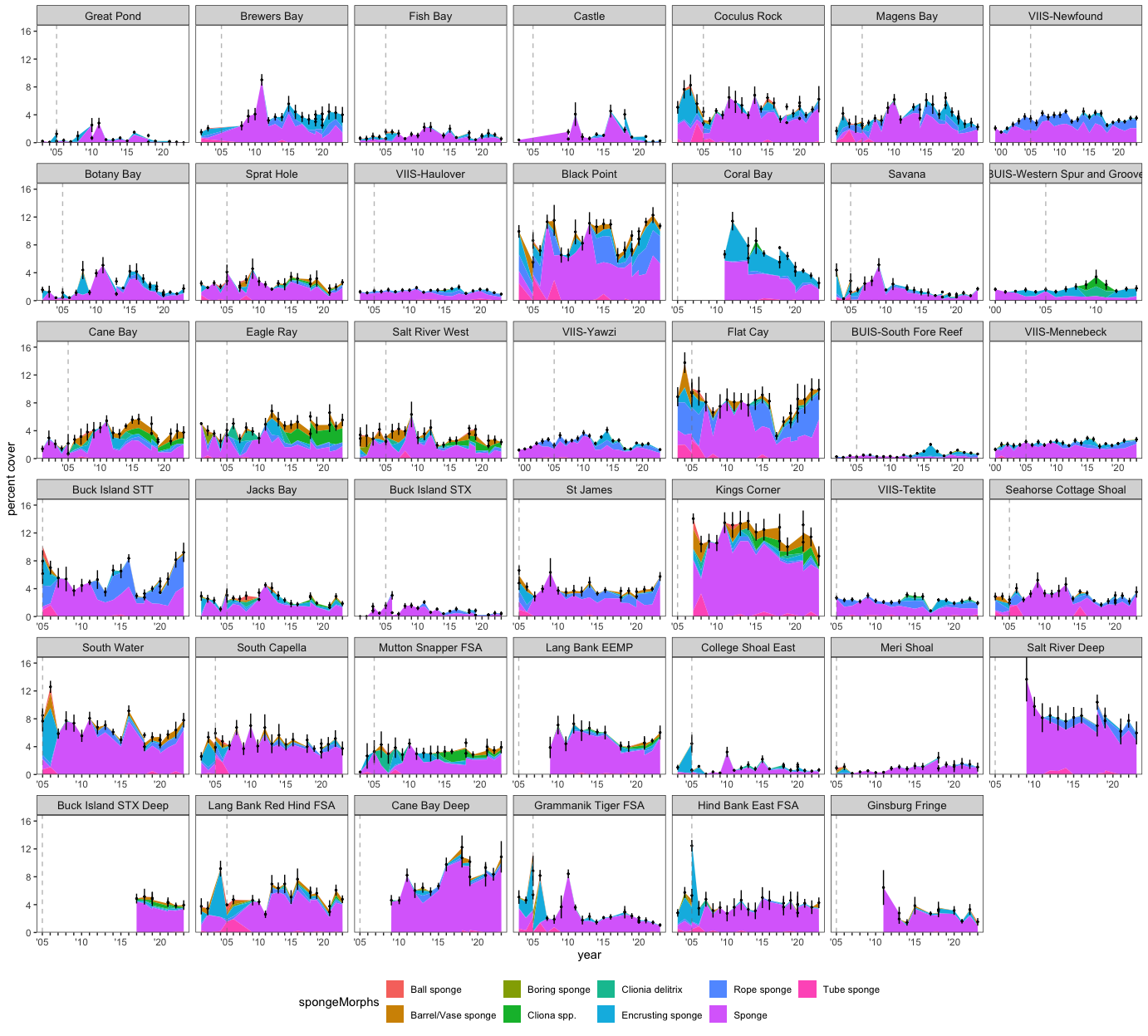

Sec 2.8 Figure 1: Percent cover of sponge morphs over time at each site, separated by sponge morph. Sites are ordered from shallow to deep. Black points show average total sponge cover +- SE. The dashed line marks the 2005 bleaching event.

Key result

Sponge morphs occupy a small share of benthic cover relative to coral and algae, so the stacked areas stay low across most sites. The site facets show which morphs are present at each depth and how total sponge cover shifts through the record, with TCRMP sites carrying the earliest years before VINPS surveys begin.

Export and download the data

What happens here: the page writes the long-format sponge-morph cover table and its metadata to the shared outputs folder, then offers both plus the page source for download.

The sponge-morph cover table (s2pt8_benthicCoverSpongeMorphs), its metadata, and this page’s .qmd source download below.

2.8 Percentage cover of sponge morphs

On this page

Data sources

Load workspace and define variables

Reorganize benthicDat into subgroupings of interest

getBenthicDatColInds()

makeGroupedBenthicDat()

merge the benthicDat from three programs

Summarize and plot

Annual percentage total sponge cover

Annual percentage cover of sponge morphs

Plot

Export and download the data

Reorganize `benthicDat` into subgroupings of interest

`getBenthicDatColInds()`

`makeGroupedBenthicDat()`

merge the `benthicDat` from three programs