 [1] "mod_coralcover_relative"         "mod_coralcover_relativeRecovery"
 [3] "predisturbance_interval"         "recovery_interval"
 [5] "resistance_year"                 "section"
 [7] "set_maxyear"                     "set_minyear"
 [9] "sitedat"                         "summary_coralcover_absreldiv"
benthic cover
about
2.1 Reformat raw benthic cover data
2.2 Cross-reference benthic codes
2.3 percentage cover of main benthic categories
2.4 percentage cover of coral genera
2.5 percentage cover of coral species
2.6 percentage cover of coral trait groups
2.7 percentage cover of algae taxa
2.8 percentage cover of sponge morphs
2.9 percentage cover of zoanthids and gorgonians
2.10 percentage cover of other benthic categories
VI Reef Resilience Study
(Any Others?)
5.2 Resilience classification based on coral cover
On this page
This page processes the summary_coralcover_absreldiv dataset to classify reef sites by their ability to resist and recover from disturbance. It labels each site “Resistant” based on relative coral cover immediately after the 2005 disturbance, and then, for non-resistant sites, further classifies them as “Nonresistant/Recovered” or “Nonresistant/Nonrecovered” based on coral cover trends through the recovery period. It produces a resilience-classified coral cover product and a relative-recovery product, both available in the Downloads section below.
Data sources
This page reads the coral cover workspace derived in section 5.1, which draws on benthic cover data from the TCRMP, VINPS, and CSUN monitoring programs. The resilience-classified cover product and the relative-recovery product derived here are available in the Downloads section below.
Load workspace and define some variables
Load the coral cover data output from part 1 coral cover data calculations.
Interactive dashboard
Explore the full site-by-year coral-cover series that feeds the resilience classification. The plot shows mean percent coral cover through time for the sites with highest cover; the table is the complete dataset (every site and year), searchable and filterable.
Classify resilience status
This code performs a classification of reef sites based on their resilience status following certain criteria, using the summary_coralcover_absreldiv dataset. Here’s a concise summary:
data_recover: isolates summary_coralcover_absreldiv for the years 2007 to 2024. For each site:
A linear model is fitted to determine the relationship between the year and
mean_coralcover_relative.The slope of the relationship (indicating the trend of coral cover over time) and its significance (p-value) are calculated.
The number of years with a positive
mean_coralcover_relativevalue is counted for each site.-
Based on the derived metrics, sites are classified into:
-
“Nonresistant/Recovered” if either:
- The slope is positive and statistically significant (p < 0.05).
- The count of positive
mean_coralcover_relativevalues exceeds 0.
“Nonresistant/Nonrecovered” for all other sites.
-
data_resist: isolates summary_coralcover_absreldiv dataset for the year 2006:
It first filters the data to retain only entries from 2006
Sites are immediately classified as either “Resistant” (if their
mean_coralcover_relativevalue is greater than 0) or “Non-Resistant”.This preliminary classification is then combined with the
data_recoverdataset, which contains the recovery status (“Nonresistant/Recovered” or “Nonresistant/Nonrecovered”) for each site.-
A final resilience status is determined:
- “Resistant” sites retain their classification.
- “Non-Resistant” sites inherit their recovery status from the
data_recoverdataset.
The final output consists of each site’s name and its corresponding resilience classification.
Show code
# Per-site recovery trend. Fit a linear slope only where a site has enough data
# (>=3 records over >=2 distinct years); sparser sites get NA slope/p and fall
# through to the "any positive years" rule, so no site crashes the fit.
.fit_site <- function(d) {
  d <- d[is.finite(d$mean_coralcover_relative) & is.finite(d$year), ]
  if (nrow(d) >= 3 && length(unique(d$year)) >= 2) {
    sm <- summary(lm(mean_coralcover_relative ~ year, data = d))$coefficients
    if ("year" %in% rownames(sm))
      return(data.frame(slope = sm["year", "Estimate"], p = sm["year", "Pr(>|t|)"]))
  }
  data.frame(slope = NA_real_, p = NA_real_)
}

data_recover <-
  summary_coralcover_absreldiv |>
  filter(year %in% recovery_interval[1]:recovery_interval[2]) |>
  group_by(site) |>
  group_modify(~ cbind(
    .fit_site(.x),
    positive_values_count = sum(.x$mean_coralcover_relative > 0, na.rm = TRUE)
  )) |>
  ungroup() |>
  mutate(
    recovery_status = if_else(
      (!is.na(slope) & slope > 0 & !is.na(p) & p < 0.05) | positive_values_count > 0,
      "Nonresistant/Recovered",
      "Nonresistant/Nonrecovered"
    )
  ) |>
  select(site, recovery_status)

# classify resistance status and combine
data_resist <- summary_coralcover_absreldiv |>
  filter(year == resistance_year) |>
  left_join(data_recover,
            by = "site") |>
  mutate(resilience = if_else(mean_coralcover_relative > 0, "Resistant", recovery_status)) |>
  select(site, resilience)

# Create a formatted table using 'kbl', set table properties, and create a scrollable box for the table
kbl(data_resist) |>
  kable_paper(full_width = F) |>
  kable_styling(
    fixed_thead = T,
    bootstrap_options = c("hover", "condensed"),
    font_size = 8
  ) |>
scroll_box(width = "75%", height = "250px")| site | resilience |
|---|---|
| BUIS-South Fore Reef | Nonresistant/Recovered |
| BUIS-Western Spur and Groove | Nonresistant/Nonrecovered |
| Black Point | Nonresistant/Recovered |
| Botany Bay | Nonresistant/Nonrecovered |
| Buck Island STT | Resistant |
| Buck Island STX | Nonresistant/Nonrecovered |
| Cabritte Horn | Resistant |
| Cane Bay | Nonresistant/Nonrecovered |
| Coculus Rock | Resistant |
| College Shoal East | Nonresistant/Recovered |
| Eagle Ray | Nonresistant/Recovered |
| East Tektite | Nonresistant/Nonrecovered |
| Europa Bay | Nonresistant/Recovered |
| Fish Bay | Nonresistant/Nonrecovered |
| Flat Cay | Nonresistant/Recovered |
| Grammanik Tiger FSA | Nonresistant/Nonrecovered |
| Great Pond | Nonresistant/Nonrecovered |
| Hind Bank East FSA | Nonresistant/Recovered |
| Jacks Bay | Nonresistant/Nonrecovered |
| Lang Bank Red Hind FSA | Resistant |
| Magens Bay | Resistant |
| Meri Shoal | NA |
| Mutton Snapper FSA | Nonresistant/Nonrecovered |
| Salt River West | Nonresistant/Recovered |
| Savana | Nonresistant/Nonrecovered |
| Seahorse Cottage Shoal | Nonresistant/Nonrecovered |
| South Capella | Nonresistant/Nonrecovered |
| South Water | Resistant |
| St James | Nonresistant/Recovered |
| Tektite | Nonresistant/Nonrecovered |
| VIIS-Haulover | Nonresistant/Nonrecovered |
| VIIS-Mennebeck | Nonresistant/Nonrecovered |
| VIIS-Newfound | Nonresistant/Nonrecovered |
| VIIS-Tektite | NA |
| VIIS-Yawzi | Nonresistant/Recovered |
| West Little Lameshur | Nonresistant/Nonrecovered |
| West Tektite | Nonresistant/Recovered |
| White Point | Nonresistant/Recovered |
| Yawzi | Nonresistant/Nonrecovered |
now combine back to summary_coralcover_absreldiv
also change resilience names for more streamlined classification
Show code
summary_coralcover_absreldiv <-
  summary_coralcover_absreldiv |>
  left_join(data_resist, by = "site") |>
  filter(!is.na(resilience)) |>
  mutate(resilience2 =
           if_else(
             resilience == "Nonresistant/Recovered",
             "recover",
             if_else(resilience == "Nonresistant/Nonrecovered",
                     "none",
                     "resist")
           )) |>
  mutate(resilience = resilience2) |>
  select(-resilience2)

summary_coralcover_absreldiv$resilience <-
  factor(summary_coralcover_absreldiv$resilience,
         levels = c("none", "recover", "resist"))
initial coral cover
Show code
library(ggrepel)

summary_coralcover_absreldiv |>
  group_by(resilience, site, depth) |>
  summarise(coralCoverPreDisturbance = min(coralCoverPreDisturbance)) |>
  ggplot(aes(x=resilience, y=coralCoverPreDisturbance)) +
  geom_violin(fill="gray75",color="white") +
  geom_boxplot(width=0.1,color="gray50")+
  geom_point(aes(group=depth,color=depth)) +
  geom_text_repel(aes(label=site, color = depth), size = 3) +
  scale_color_continuous(low="cyan",high="purple")+
  scale_fill_continuous(low="red",high="purple")+
  theme_bw() +
  labs(y = "Average of pre-disturbance coral cover", x = "resilience")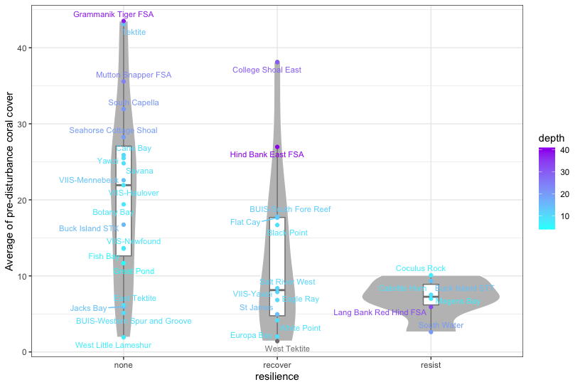
apparently “resistant” sites tended towards lower pre-disturbance coral cover ( < 10%) .
Plot
Show code
df <- summary_coralcover_absreldiv

set_minyear <- min(df$year)
set_maxyear <- max(df$year)

df <- df |>
  group_by(site) |>
  mutate(mean_coraldiversity = if_else(
    is.na(mean_coraldiversity),
    (
      lag(
        mean_coraldiversity,
        default = first(mean_coraldiversity, order_by = year)
      ) +
        lead(
          mean_coraldiversity,
          default = last(mean_coraldiversity, order_by = year)
        )
    ) / 2,
    mean_coraldiversity
  )) |>
  mutate(sd_coraldiversity = if_else(
    is.na(mean_coraldiversity),
    (
      lag(
        sd_coraldiversity,
        default = first(sd_coraldiversity, order_by = year)
      ) +
        lead(
          mean_coraldiversity,
          default = last(sd_coraldiversity, order_by = year)
        )
    ) / 2,
    sd_coraldiversity
  )) |>
  ungroup()

df$sd_coraldiversity[is.na(df$sd_coraldiversity)] <- 0

min_div <- min(df$mean_coraldiversity, na.rm = TRUE)
max_div <- max(df$mean_coraldiversity, na.rm = TRUE)

# Scale mean_coraldiversity to -1 to 1
df$mean_coraldiversity_scaled <-
  2 * (df$mean_coraldiversity - min_div) / (max_div - min_div) - 1

my_colors <- rainbow(5)

fillmin <- min(df$mean_coralcover)
fillmax <- max(df$mean_coralcover)


pfunction <- function(name, nrowf, ncolf) {
  p <- ggplot(
    df |> filter(resilience == name),
    aes(
      x = year,
      y = mean_coralcover_relative,
      shape = status,
      group = site
    )
  ) +
    geom_hline(yintercept = 0,
               color = "black",
               size = 0.25)

  # Adding second axis with transformed data
  p <- p +
    geom_line(
      aes(y = mean_coraldiversity_scaled),
      color = "grey50",
      alpha = 0.25,
      linewidth = 0.5
    ) +
    # geom_point(aes(y = mean_coraldiversity_scaled), color = "grey50", shape = 4,size=2) +
    geom_ribbon(aes(
      ymin = 2 * (mean_coraldiversity - sd_coraldiversity - min_div) / (max_div - min_div) - 1,
      ymax = 2 * (mean_coraldiversity + sd_coraldiversity - min_div) / (max_div - min_div) - 1
    ),
    fill = "grey50",
    alpha = 0.20) +
    scale_y_continuous(
      sec.axis = sec_axis(
        ~ .x,
        breaks = c(-1, 1),
        labels = c(round(min_div, 0), round(max_div, 0)),
        name = "coral diversity (inverse simpsons D of coral genera"
      )
    )

  #adding coral cover percentages back on top
  p <- p +
    geom_line(color = "black") +
    geom_errorbar(
      aes(
        ymin = mean_coralcover_relative - sd_coralcover_relative,
        ymax = mean_coralcover_relative + sd_coralcover_relative
      ),
      color = "black",
      width = 0.1,
      size = 0.5
    ) +
    geom_point(
      aes(fill = mean_coralcover),
      size = 3,
      color = "black",
      alpha = 1
    ) +
    scale_shape_manual(values = c(21, 25, 24), name = "relative status") +
    scale_fill_gradientn(
      limits = c(fillmin, fillmax),
      colors =  my_colors,
      name = "annual % coral cover"
    ) +
    facet_wrap(~ site, ncol = ncolf) +   # rows auto-computed so any per-class site count fits
    ylab("percentage coral cover relative to pre-disturbance") +
    coord_cartesian(ylim = c(-1, 1)) +
    scale_x_continuous(
      expand = c(0, 0),
      limits = c(set_minyear - 0.4, set_maxyear + 0.4),
      breaks = seq(set_minyear, set_maxyear, by = 1),
      name = "year"
    ) +
    theme_bw() +
    theme(strip.text = element_text(size = 10)) +
    theme(legend.position = "bottom") +
    theme(panel.grid.major = element_blank(),
          panel.grid.minor = element_blank()) +
    theme(axis.text.x = element_text(
      angle = 90,
      vjust = 0.5,
      hjust = 1
    )) +
    theme(axis.title.y.right = element_text(
      angle = 90,
      vjust = 0.5,
      hjust = 0.5
    )) +
    theme(
      axis.line.y.right = element_line(color = "grey50", size = 1),
      axis.ticks.y.right = element_line(color = "grey50"),
      axis.text.y.right = element_text(color = "grey50"),
      axis.title.y.right = element_text(color = "grey50")
    )
  return(p)
}


presist <-
  pfunction("resist", 2, 2) +
  theme(
    # legend.position = "top",
    axis.title.x = element_blank(),
    axis.text.x = element_blank(),
    axis.title.y = element_blank(),
    axis.title.y.right = element_blank()
  ) +
  ggtitle("Resistant sites") +
  theme(legend.direction = "horizontal", legend.box = "vertical")

precover <- pfunction("recover", 3, 5) +
  theme(
    legend.position = "none",
    axis.title.x = element_blank(),
    axis.text.x = element_blank(),
    axis.title.y = element_blank(),
    axis.title.y.right = element_blank()
  ) +
  ggtitle("Recovered or recovering sites")

pnone <- pfunction("none", 4, 5) +
  theme(legend.position = "none") +
  # axis.title.x = element_blank(),
  # axis.title.y = element_blank(),
  # axis.title.y.right = element_blank()) +
  ggtitle("Sites that neither resisted nor recovered")

library(patchwork)

(presist + guide_area() + plot_layout(widths = c(2, 3), guides = 'collect')) / precover / pnone +
  plot_layout(heights = c(2, 3, 3))

svg(filename = "resilience.svg",
    width = 13,
    height = 13)

(presist + guide_area() + plot_layout(widths = c(2, 3), guides = 'collect')) / precover / pnone +
  plot_layout(heights = c(2, 3, 3))

dev.off()
quartz_off_screen
2 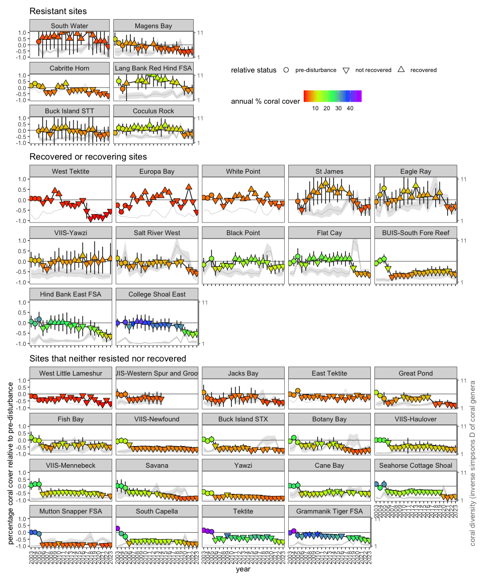
Join resilience categories to mod_coralcover_relative for export
Provenance
Write the resilience-classified cover product and the relative-recovery product, each with its metadata sidecar, to outputs/. This block is hidden from the page (echo/output false) because it is plumbing, not analysis. The writes still run on every render.